R語言 | 關聯規則

阿新 • • 發佈：2019-01-10

1.概念

1.1 引論

關聯規則（AssociationRules）是無監督的機器學習方法，用於知識發現，而非預測。

關聯規則的學習器（learner）無需事先對訓練資料進行打標籤，因為無監督學習沒有訓練這個步驟。缺點是很難對關聯規則學習器進行模型評估，一般都可以通過肉眼觀測結果是否合理。

關聯規則主要用來發現Pattern，最經典的應用是購物籃分析，當然其他類似於購物籃交易資料的案例也可以應用關聯規則進行模式發現，如電影推薦、約會網站或者藥物間的相互副作用。

1.2 例子 - 源資料

點選流資料。

不同的Session訪問的新聞版塊，如下所示：

Session ID	List of media categories accessed
1	{News, Finance}
2	{News, Finance}
3	{Sports, Finance, News}
4	{Arts}
5	{Sports, News, Finance}
6	{News, Arts, Entertainment}

1.3資料格式

關聯規則需要把源資料的格式轉換為稀疏矩陣。

把上表轉化為稀疏矩陣，1表示訪問，0表示未訪問。

Session ID	News	Finance	Entertainment	Sports
1	1	1	0	0
2	1	1	0	0
3	1	1	0	1
4	0	0	0	0
5	1	1	0	1
6	1	0	1	0

1.4術語和度量

1.4.1項集 ItemSet

這是一條關聯規則：

括號內的Item集合稱為項集。如上例，{News, Finance}是一個項集，{Sports}也是一個項集。

這個例子就是一條關聯規則：基於歷史記錄，同時看過News和Finance版塊的人很有可能會看Sports版塊。

{News,Finance} 是這條規則的Left-hand-side (LHS or Antecedent)

{Sports}是這條規則的Right-hand-side (RHS or Consequent)

LHS（Left Hand Side)的項集和RHS（Right Hand Side）的項集不能有交集。

下面介紹衡量關聯規則強度的度量。

1.4.2支援度 Support

項集的支援度就是該項集出現的次數除以總的記錄數（交易數）。

Support({News}) = 5/6 = 0.83

Support({News, Finance}) = 4/6 =0.67

Support({Sports}) = 2/6 = 0.33

支援度的意義在於度量項集在整個事務集中出現的頻次。我們在發現規則的時候，希望關注頻次高的項集。

1.4.3置信度 Confidence

關聯規則 X -> Y 的置信度計算公式

規則的置信度的意義在於項集{X，Y}同時出現的次數佔項集{X}出現次數的比例。發生X的條件下，又發生Y的概率。

表示50%的人訪問過{News, Finance}，同時也會訪問{Sports}

1.4.4提升度 Lift

當右手邊的項集（consequent）的支援度已經很顯著時，即時規則的Confidence較高，這條規則也是無效的。

舉個例子：

在所分析的10000個事務中,6000個事務包含計算機遊戲,7500個包含遊戲機遊戲,4000個事務同時包含兩者。

關聯規則（計算機遊戲，遊戲機遊戲）支援度為0.4，看似很高，但其實這個關聯規則是一個誤導。

在使用者購買了計算機遊戲後有（4000÷6000）0.667 的概率的去購買遊戲機遊戲，而在沒有任何前提條件時，使用者反而有（7500÷10000）0.75的概率去購買遊戲機遊戲，也就是說設定了購買計算機遊戲這樣的條件反而會降低使用者去購買遊戲機遊戲的概率，所以計算機遊戲和遊戲機遊戲是相斥的。

所以要引進Lift這個概念，Lift(X->Y)=Confidence(X->Y)/Support(Y)

規則的提升度的意義在於度量項集{X}和項集{Y}的獨立性。即，Lift(X->Y)= 1 表面 {X}，{Y}相互獨立。[注：P(XY)=P(X)*P(Y),if X is independent of Y]

如果該值=1,說明兩個條件沒有任何關聯,如果<1,說明A條件(或者說A事件的發生)與B事件是相斥的,一般在資料探勘中當提升度大於3時,我們才承認挖掘出的關聯規則是有價值的。

最後，lift(X->Y) = lift(Y->X)

1.4.5出錯率 Conviction

Conviction的意義在於度量規則預測錯誤的概率。

表示X出現而Y不出現的概率。

例子：

表面這條規則的出錯率是32%。

1.5生成規則

一般兩步：

第一步，找出頻繁項集。n個item，可以產生2^n- 1 個項集（itemset）。所以，需要指定最小支援度，用於過濾掉非頻繁項集。
第二部，找出第一步的頻繁項集中的規則。n個item，總共可以產生3^n - 2^(n+1) + 1條規則。所以，需要指定最小置信度，用於過濾掉弱規則。

第一步的計算量比第二部的計算量大。

2.Apriori演算法

Apriori Principle

如果項集A是頻繁的，那麼它的子集都是頻繁的。如果項集A是不頻繁的，那麼所有包括它的父集都是不頻繁的。

例子：{X, Y}是頻繁的，那麼{X}，{Y}也是頻繁的。如果{Z}是不頻繁的，那麼{X,Z}, {Y, Z}, {X, Y, Z}都是不頻繁的。

生成頻繁項集

給定最小支援度Sup，計算出所有大於等於Sup的項集。

第一步，計算出單個item的項集，過濾掉那些不滿足最小支援度的項集。

第二步，基於第一步，生成兩個item的項集，過濾掉那些不滿足最小支援度的項集。

第三步，基於第二步，生成三個item的項集，過濾掉那些不滿足最小支援度的項集。

如下例子：

One-Item Sets	Support Count	Support
{News}	5	0.83
{Finance}	4	0.67
{Entertainment}	1	0.17
{Sports}	2	0.33
Two-Item Sets	Support Count	Support
{News, Finance}	4	0.67
{News, Sports}	2	0.33
{Finance, Sports}	2	0.33
Three-Item Sets	Support Count	Support
{News, Finance, Sports}	2	0.33

規則生成

給定Confidence、Lift 或者 Conviction，基於上述生成的頻繁項集，生成規則，過濾掉那些不滿足目標度量的規則。因為規則相關的度量都是通過支援度計算得來，所以這部分過濾的過程很容易完成。

Apriori案例分析（R語言）

1. 關聯規則的包

arules是用來進行關聯規則分析的R語言包。

library(arules)

2. 載入資料集

源資料：groceries 資料集，每一行代表一筆交易所購買的產品（item）

資料轉換：建立稀疏矩陣，每個Item一列，每一行代表一個transaction。1表示該transaction購買了該item，0表示沒有購買。當然，data frame是比較直觀的一種資料結構，但是一旦item比較多的時候，這個data frame的大多數單元格的值為0，大量浪費記憶體。所以，R引入了特殊設計的稀疏矩陣，僅存1，節省記憶體。arules包的函式read.transactions可以讀入源資料並建立稀疏矩陣。

groceries <- read.transactions("groceries.csv", format="basket", sep=",")

引數說明：

format=c("basket", "single")用於註明源資料的格式。如果源資料每行內容就是一條交易購買的商品列表（類似於一行就是一個購物籃）那麼使用basket；如果每行內容是交易號+單個商品，那麼使用single。

cols=c("transId", "ItemId") 對於single格式，需要指定cols，二元向量（數字或字串）。如果是字串，那麼檔案的第一行是表頭（即列名）。第一個元素是交易號的欄位名，第二個元素是商品編號的欄位名。如果是數字，那麼無需表頭。對於basket，一般設定為NULL，預設也是NULL，所以不用指定。

signle format的資料格式如下所示，與此同時，需要設定cols=c(1, 2)

1001,Fries

1001,Coffee

1001,Milk

1002,Coffee

1002,Fries

rm.duplicates=FALSE：表示對於同一交易，是否需要刪除重複的商品。

接下來，檢視資料集相關的統計彙總資訊，以及資料集本身。

summary(groceries)
transactions as itemMatrix in sparse format with
 9835 rows (elements/itemsets/transactions) and
 169 columns (items) and a density of 0.02609146 

most frequent items:
      whole milk other vegetables       rolls/buns             soda 
            2513             1903             1809             1715 
          yogurt          (Other) 
            1372            34055 

element (itemset/transaction) length distribution:
sizes
   1    2    3    4    5    6    7    8    9   10   11   12   13   14   15 
2159 1643 1299 1005  855  645  545  438  350  246  182  117   78   77   55 
  16   17   18   19   20   21   22   23   24   26   27   28   29   32 
  46   29   14   14    9   11    4    6    1    1    1    1    3    1 

   Min. 1st Qu.  Median    Mean 3rd Qu.    Max. 
  1.000   2.000   3.000   4.409   6.000  32.000 

includes extended item information - examples:
            labels
1 abrasive cleaner
2 artif. sweetener
3   baby cosmetics

summary的含義：

第一段：總共有9835條交易記錄transaction，169個商品item。density=0.026表示在稀疏矩陣中1的百分比。
第二段：最頻繁出現的商品item，以及其出現的次數。可以計算出最大支援度。

第三段：每筆交易包含的商品數目，以及其對應的5個分位數和均值的統計資訊。如：2159條交易僅包含了1個商品，1643條交易購買了2件商品，一條交易購買了32件商品。那段統計資訊的含義是：第一分位數是2，意味著25%的交易包含不超過2個item。中位數是3表面50%的交易購買的商品不超過3件。均值4.4表示所有的交易平均購買4.4件商品。

第四段：如果資料集包含除了Transaction Id 和 Item之外的其他的列（如，發生交易的時間，使用者ID等等），會顯示在這裡。這個例子，其實沒有新的列，labels就是item的名字。

進一步檢視資料集的資訊

> class(groceries)
[1] "transactions"
attr(,"package")
[1] "arules"
> groceries
transactions in sparse format with
 9835 transactions (rows) and
 169 items (columns)
> dim(groceries)
[1] 9835  169
> colnames(groceries)[1:5]
[1] "abrasive cleaner" "artif. sweetener" "baby cosmetics"   "baby food"        "bags"            
> rownames(groceries)[1:5]
[1] "1" "2" "3" "4" "5"

basketSize表示每個transaction包含item的數目，是row level。而ItemFrequency是這個item的支援度，是column level。

> basketSize<-size(groceries)
> summary(basketSize)
   Min. 1st Qu.  Median    Mean 3rd Qu.    Max. 
  1.000   2.000   3.000   4.409   6.000  32.000 
> sum(basketSize) #count of all 1s in the sparse matrix
[1] 43367
> itemFreq <- itemFrequency(groceries)
> itemFreq[1:5]
abrasive cleaner artif. sweetener   baby cosmetics        baby food             bags 
    0.0035587189     0.0032536858     0.0006100661     0.0001016777     0.0004067107 
> sum(itemFreq) #本質上代表"平均一個transaction購買的item個數"
[1] 4.409456

可以檢視basketSize的分佈：密度曲線(TO ADD HERE)

itemCount表示每個item出現的次數。Support(X) = Xs / N, N是總的交易數，Xs就是Item X的count。

itemXCount = N * itemXFreq = (ItemXFreq / sum(itemFreq)) * sum(basketSize)

> itemCount <- (itemFreq/sum(itemFreq))*sum(basketSize)
> summary(itemCount)
   Min. 1st Qu.  Median    Mean 3rd Qu.    Max. 
    1.0    38.0   103.0   256.6   305.0  2513.0 
> orderedItem <- sort(itemCount, decreasing = )
> orderedItem <- sort(itemCount, decreasing = T)
> orderedItem[1:10]
      whole milk other vegetables       rolls/buns             soda           yogurt    bottled water 
            2513             1903             1809             1715             1372             1087 
 root vegetables   tropical fruit    shopping bags          sausage 
            1072             1032              969              924

當然，也可以把支援度itemFrequency排序，檢視支援度的最大值

> orderedItemFreq <- sort(itemFrequency(groceries), decreasing=T)
> orderedItemFreq[1:10]
      whole milk other vegetables       rolls/buns             soda           yogurt    bottled water 
      0.25551601       0.19349263       0.18393493       0.17437722       0.13950178       0.11052364 
 root vegetables   tropical fruit    shopping bags          sausage 
      0.10899847       0.10493137       0.09852567       0.09395018

如果要切一塊子集出來計算支援度，可以對資料集進行矩陣行列下標操作。

如下例，切除第100行到800行，計算第1列到第3列的支援度。也就是說，資料集通過向量的下標按行切，也可以通過矩陣下標按行列切。

> itemFrequency(groceries[100:800,1:3])
abrasive cleaner artif. sweetener   baby cosmetics 
     0.005706134      0.001426534      0.001426534

可以通過圖形更直觀觀測。

按最小支援度檢視。

> itemFrequencyPlot(groceries, support=0.1)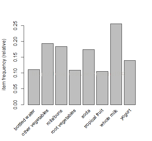

按照排序檢視。

> itemFrequencyPlot(groceries, topN=10, horiz=T)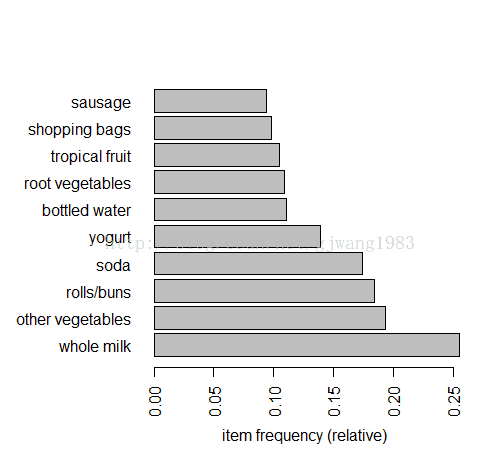

最後，可以根據業務對資料集進行過濾，獲得進一步規則挖掘的資料集。如下例，只關心購買兩件商品以上的交易。

> groceries_use <- groceries[basketSize > 1]
> dim(groceries_use)
[1] 7676  169

檢視資料

inspect(groceries[1:5])
  items                     
1 {citrus fruit,            
   margarine,               
   ready soups,             
   semi-finished bread}     
2 {coffee,                  
   tropical fruit,          
   yogurt}                  
3 {whole milk}              
4 {cream cheese,            
   meat spreads,            
   pip fruit,               
   yogurt}                  
5 {condensed milk,          
   long life bakery product,
   other vegetables,        
   whole milk}

也可以通過圖形更直觀觀測資料的稀疏情況。一個點代表在某個transaction上購買了item。

> image(groceries[1:10])

當資料集很大的時候，這張稀疏矩陣圖是很難展現的，一般可以用sample函式進行取樣顯示。

> image(sample(groceries,100))

這個矩陣圖雖然看上去沒有包含很多資訊，但是它對於直觀地發現異常資料或者比較特殊的Pattern很有效。比如，某些item幾乎每個transaction都會買。比如，聖誕節都會買糖果禮物。那麼在這幅圖上會顯示一根豎線，在糖果這一列上。

給出一個通用的R函式，用於顯示如上所有的指標：

library(arules)  # association rules
library(arulesViz)  # data visualization of association rules
library(RColorBrewer)  # color palettes for plots

3. 進行規則挖掘

為了進行規則挖掘，第一步是設定一個最小支援度，這個最小支援度可以由具體的業務規則確定。

介紹apriori函式的用法：

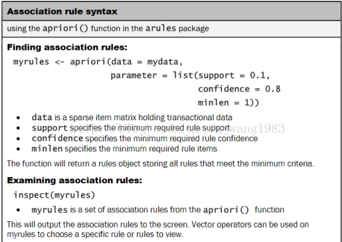
這裡需要說明下parameter：

預設的support=0.1, confidence=0.8, minlen=1, maxlen=10

對於minlen，maxlen這裡指規則的LHS+RHS的並集的元素個數。所以minlen=1，意味著 {} => {beer}是合法的規則。我們往往不需要這種規則，所以需要設定minlen=2。

> groceryrules <- apriori(groceries, parameter = list(support =
+                                                         0.006, confidence = 0.25, minlen = 2))

Parameter specification:
 confidence minval smax arem  aval originalSupport support minlen maxlen target   ext
       0.25    0.1    1 none FALSE            TRUE   0.006      2     10  rules FALSE

Algorithmic control:
 filter tree heap memopt load sort verbose
    0.1 TRUE TRUE  FALSE TRUE    2    TRUE

apriori - find association rules with the apriori algorithm
version 4.21 (2004.05.09)        (c) 1996-2004   Christian Borgelt
set item appearances ...[0 item(s)] done [0.00s].
set transactions ...[169 item(s), 9835 transaction(s)] done [0.00s].
sorting and recoding items ... [109 item(s)] done [0.00s].
creating transaction tree ... done [0.00s].
checking subsets of size 1 2 3 4 done [0.01s].
writing ... [463 rule(s)] done [0.00s].
creating S4 object  ... done [0.00s].

從返回的結果看，總共有463條規則生成。

評估模型

使用summary函式檢視規則的彙總資訊。

> summary(groceryrules)
set of 463 rules

rule length distribution (lhs + rhs):sizes
  2   3   4 
150 297  16 

   Min. 1st Qu.  Median    Mean 3rd Qu.    Max. 
  2.000   2.000   3.000   2.711   3.000   4.000 

summary of quality measures:
    support           confidence          lift       
 Min.   :0.006101   Min.   :0.2500   Min.   :0.9932  
 1st Qu.:0.007117   1st Qu.:0.2971   1st Qu.:1.6229  
 Median :0.008744   Median :0.3554   Median :1.9332  
 Mean   :0.011539   Mean   :0.3786   Mean   :2.0351  
 3rd Qu.:0.012303   3rd Qu.:0.4495   3rd Qu.:2.3565  
 Max.   :0.074835   Max.   :0.6600   Max.   :3.9565  

mining info:
      data ntransactions support confidence
 groceries          9835   0.006       0.25

第一部分：規則的長度分佈：就是minlen到maxlen之間的分佈。如上例，len=2有150條規則，len=3有297，len=4有16。同時，rule length的五數分佈+均值。

第二部分：quality measure的統計資訊。

第三部分：挖掘的相關資訊。

使用inpect檢視具體的規則。

> inspect(groceryrules[1:5])
  lhs                rhs                    support confidence     lift
1 {potted plants} => {whole milk}       0.006914082  0.4000000 1.565460
2 {pasta}         => {whole milk}       0.006100661  0.4054054 1.586614
3 {herbs}         => {root vegetables}  0.007015760  0.4312500 3.956477
4 {herbs}         => {other vegetables} 0.007727504  0.4750000 2.454874
5 {herbs}         => {whole milk}       0.007727504  0.4750000 1.858983

4. 評估規則

規則可以劃分為3大類：

Actionable
- 這些rule提供了非常清晰、有用的洞察，可以直接應用在業務上。

Trivial
- 這些rule顯而易見，很清晰但是沒啥用。屬於common sense，如 {尿布} => {嬰兒食品}。

Inexplicable
- 這些rule是不清晰的，難以解釋，需要額外的研究來判定是否是有用的rule。

接下來，我們討論如何發現有用的rule。

按照某種度量，對規則進行排序。

> ordered_groceryrules <- sort(groceryrules, by="lift")
> inspect(ordered_groceryrules[1:5])
  lhs                   rhs                      support confidence     lift
1 {herbs}            => {root vegetables}    0.007015760  0.4312500 3.956477
2 {berries}          => {whipped/sour cream} 0.009049314  0.2721713 3.796886
3 {other vegetables,                                                        
   tropical fruit,                                                          
   whole milk}       => {root vegetables}    0.007015760  0.4107143 3.768074
4 {beef,                                                                    
   other vegetables} => {root vegetables}    0.007930859  0.4020619 3.688692
5 {other vegetables,                                                        
   tropical fruit}   => {pip fruit}          0.009456024  0.2634561 3.482649

搜尋規則

> yogurtrules <- subset(groceryrules, items %in% c("yogurt"))
> inspect(yogurtrules)
    lhs                        rhs                    support confidence     lift
1   {cat food}              => {yogurt}           0.006202339  0.2663755 1.909478
2   {hard cheese}           => {yogurt}           0.006405694  0.2614108 1.873889
3   {butter milk}           => {yogurt}           0.008540925  0.3054545 2.189610
......
18  {cream cheese,                                                               
     yogurt}                => {whole milk}       0.006609049  0.5327869 2.085141
......
121 {other vegetables,                                                           
     whole milk}            => {yogurt}           0.022267412  0.2975543 2.132979

items %in% c("A", "B")表示 lhs+rhs的項集並集中，至少有一個item是在c("A", "B")。 item = Aor item = B

如果僅僅想搜尋lhs或者rhs，那麼用lhs或rhs替換items即可。如：lhs %in% c("yogurt")

%in%是精確匹配

%pin%是部分匹配，也就是說只要item like '%A%' or item like '%B%'

%ain%是完全匹配，也就是說itemset has ’A' and itemset has ‘B'

同時可以通過條件運算子(&, |, !) 新增 support, confidence, lift的過濾條件。

例子如下：

> fruitrules <- subset(groceryrules, items %pin% c("fruit"))
> inspect(fruitrules)
    lhs                        rhs                    support confidence     lift
1   {grapes}                => {tropical fruit}   0.006100661  0.2727273 2.599101
2   {fruit/vegetable juice} => {soda}             0.018403660  0.2545710 1.459887

> byrules <- subset(groceryrules, items %ain% c("berries", "yogurt"))
> inspect(byrules)
  lhs          rhs         support confidence     lift
1 {berries} => {yogurt} 0.01057448  0.3180428 2.279848

> fruitrules <- subset(groceryrules, items %pin% c("fruit") & lift > 2)
> inspect(fruitrules)
   lhs                        rhs                    support confidence     lift
1  {grapes}                => {tropical fruit}   0.006100661  0.2727273 2.599101
2  {pip fruit}             => {tropical fruit}   0.020437214  0.2701613 2.574648
3  {tropical fruit}        => {yogurt}           0.029283172  0.2790698 2.000475
4  {curd,                                                                       
    tropical fruit}        => {whole milk}       0.006507372  0.6336634 2.479936
5  {butter,                                                                     
    tropical fruit}        => {whole milk}       0.006202339  0.6224490 2.436047

檢視其它的quality measure

<span style="font-family: sans-serif; background-color: rgb(255, 255, 255);"></span><pre name="code" class="java">> qualityMeasures <- interestMeasure(groceryrules, method=c("coverage","fishersExactTest","conviction", "chiSquared"), transactions=groceries)
> summary(qualityMeasures)
    coverage        fishersExactTest      conviction       chiSquared      
 Min.   :0.009964   Min.   :0.0000000   Min.   :0.9977   Min.   :  0.0135  
 1st Qu.:0.018709   1st Qu.:0.0000000   1st Qu.:1.1914   1st Qu.: 32.1179  
 Median :0.024809   Median :0.0000000   Median :1.2695   Median : 58.4354  
 Mean   :0.032608   Mean   :0.0057786   Mean   :1.3245   Mean   : 70.4249  
 3rd Qu.:0.035892   3rd Qu.:0.0000001   3rd Qu.:1.4091   3rd Qu.: 97.1387  
 Max.   :0.255516   Max.   :0.5608331   Max.   :2.1897   Max.   :448.5699  
> quality(groceryrules) <- cbind(quality(groceryrules), qualityMeasures)
> inspect(head(sort(groceryrules, by = "conviction", decreasing = F)))
  lhs                      rhs              support confidence      lift conviction chiSquared   coverage fishersExactTest
1 {bottled beer}        => {whole milk} 0.020437214  0.2537879 0.9932367  0.9976841 0.01352288 0.08052872        0.5608331
2 {bottled water,                                                                                                         
   soda}                => {whole milk} 0.007524148  0.2596491 1.0161755  1.0055826 0.02635700 0.02897814        0.4586202
3 {beverages}           => {whole milk} 0.006812405  0.2617188 1.0242753  1.0084016 0.05316028 0.02602949        0.4329533
4 {specialty chocolate} => {whole milk} 0.008032537  0.2642140 1.0340410  1.0118214 0.12264445 0.03040163        0.3850343
5 {candy}               => {whole milk} 0.008235892  0.2755102 1.0782502  1.0275976 0.63688634 0.02989324        0.2311769
6 {sausage,                                                                                                               
   soda}                => {whole milk} 0.006710727  0.2761506 1.0807566  1.0285068 0.54827850 0.02430097        0.2508610

第三個引數transactions：一般情況下都是原來那個資料集，但也有可能是其它資料集，用於檢驗這些rules在其他資料集上的效果。所以，這也是評估rules的一種方法：在其它資料集上計算這些規則的quality measure用以評估效果。

fishersExactTest 的p值大部分都是很小的（p < 0.05），這就說明這些規則反應出了真實的使用者的行為模式。

coverage從0.01 ~ 0.26，相當於覆蓋到了多少範圍的使用者。

ChiSquared: 考察該規則的LHS和RHS是否獨立？即LHS與RHS的列聯表的ChiSquare Test。p<0.05表示獨立，否則表示不獨立。

限制挖掘的item

可以控制規則的左手邊或者右手邊出現的item，即appearance。但儘量要放低支援度和置信度。

> berriesInLHS <- apriori(groceries, parameter = list( support = 0.001, confidence = 0.1 ), appearance = list(lhs = c("berries"), default="rhs"))

Parameter specification:
 confidence minval smax arem  aval originalSupport support minlen maxlen target   ext
        0.1    0.1    1 none FALSE            TRUE   0.001      1     10  rules FALSE

Algorithmic control:
 filter tree heap memopt load sort verbose
    0.1 TRUE TRUE  FALSE TRUE    2    TRUE

apriori - find association rules with the apriori algorithm
version 4.21 (2004.05.09)        (c) 1996-2004   Christian Borgelt
set item appearances ...[1 item(s)] done [0.00s].
set transactions ...[169 item(s), 9835 transaction(s)] done [0.00s].
sorting and recoding items ... [157 item(s)] done [0.00s].
creating transaction tree ... done [0.00s].
checking subsets of size 1 2 done [0.00s].
writing ... [26 rule(s)] done [0.00s].
creating S4 object  ... done [0.00s].
> summary(berriesInLHS)
set of 26 rules

rule length distribution (lhs + rhs):sizes
 1  2 
 8 18 

   Min. 1st Qu.  Median    Mean 3rd Qu.    Max. 
  1.000   1.000   2.000   1.692   2.000   2.000 

summary of quality measures:
    support           confidence          lift      
 Min.   :0.003660   Min.   :0.1049   Min.   :1.000  
 1st Qu.:0.004601   1st Qu.:0.1177   1st Qu.:1.000  
 Median :0.007016   Median :0.1560   Median :1.470  
 Mean   :0.053209   Mean   :0.1786   Mean   :1.547  
 3rd Qu.:0.107982   3rd Qu.:0.2011   3rd Qu.:1.830  
 Max.   :0.255516   Max.   :0.3547   Max.   :3.797  

mining info:
      data ntransactions support confidence
 groceries          9835   0.001        0.1
> inspect(berriesInLHS)
   lhs          rhs                         support confidence     lift
1  {}        => {bottled water}         0.110523640  0.1105236 1.000000
2  {}        => {tropical fruit}        0.104931368  0.1049314 1.000000
3  {}        => {root vegetables}       0.108998475  0.1089985 1.000000
4  {}        => {soda}                  0.174377224  0.1743772 1.000000
5  {}        => {yogurt}                0.139501779  0.1395018 1.000000
6  {}        => {rolls/buns}            0.183934926  0.1839349 1.000000
7  {}        => {other vegetables}      0.193492628  0.1934926 1.000000
8  {}        => {whole milk}            0.255516014  0.2555160 1.000000
9  {berries} => {beef}                  0.004473818  0.1345566 2.564659
10 {berries} => {butter}                0.003762074  0.1131498 2.041888
11 {berries} => {domestic eggs}         0.003863752  0.1162080 1.831579
12 {berries} => {fruit/vegetable juice} 0.003660397  0.1100917 1.522858
13 {berries} => {whipped/sour cream}    0.009049314  0.2721713 3.796886
14 {berries} => {pip fruit}             0.003762074  0.1131498 1.495738
15 {berries} => {pastry}                0.004270463  0.1284404 1.443670
16 {berries} => {citrus fruit}          0.005388917  0.1620795 1.958295
17 {berries} => {shopping bags}         0.004982206  0.1498471 1.520894
18 {berries} => {sausage}               0.004982206  0.1498471 1.594963
19 {berries} => {bottled water}         0.004067107  0.1223242 1.106769
20 {berries} => {tropical fruit}        0.006710727  0.2018349 1.923494
21 {berries} => {root vegetables}       0.006609049  0.1987768 1.823666
22 {berries} => {soda}                  0.007320793  0.2201835 1.262685
23 {berries} => {yogurt}                0.010574479  0.3180428 2.279848
24 {berries} => {rolls/buns}            0.006609049  0.1987768 1.080691
25 {berries} => {other vegetables}      0.010269446  0.3088685 1.596280
26 {berries} => {whole milk}            0.011794611  0.3547401 1.388328

既然lhs都是一樣的，那麼只檢視rhs的itemset即可，可以如下：

> inspect(head(<strong>rhs(berriesInLHS)</strong>, n=5))
  items            
1 {bottled water}  
2 {tropical fruit} 
3 {root vegetables}
4 {soda}           
5 {yogurt}

當然，還可以使用subset進行進一步的過濾，例如，不希望看到rhs包含"root vegetables" 或 "whole milk"

> berrySub <- subset(berriesInLHS, subset = !(rhs %in% c("root vegetables", "whole milk")))
> inspect(head(rhs(sort(berrySub, by="confidence")), n=5))
  items               
1 {yogurt}            
2 {other vegetables}  
3 {whipped/sour cream}
4 {soda}              
5 {tropical fruit}    
> berrySub
set of 22 rules

儲存挖掘的結果

有兩種使用場景。

第一，儲存到檔案。可以與外部程式進行交換。

> write(groceryrules, file="groceryrules.csv", sep=",", quote=TRUE, row.names=FALSE)

第二，轉換為data frame，然後再進行進一步的處理。處理完的結果可以儲存到外部檔案或者資料庫。

> groceryrules_df <- as(groceryrules, "data.frame")
> str(groceryrules_df)
'data.frame':	463 obs. of  8 variables:
 $ rules           : Factor w/ 463 levels "{baking powder} => {other vegetables}",..: 340 302 207 206 208 341 402 21 139 140 ...
 $ support         : num  0.00691 0.0061 0.00702 0.00773 0.00773 ...
 $ confidence      : num  0.4 0.405 0.431 0.475 0.475 ...
 $ lift            : num  1.57 1.59 3.96 2.45 1.86 ...
 $ conviction      : num  1.24 1.25 1.57 1.54 1.42 ...
 $ chiSquared      : num  19 17.7 173.9 82.6 41.2 ...
 $ coverage        : num  0.0173 0.015 0.0163 0.0163 0.0163 ...
 $ fishersExactTest: num  2.20e-05 4.13e-05 6.17e-26 4.56e-16 1.36e-09 ...

關於關聯規則挖掘的進階部分

1. 帶有Hierarchy的item

這裡我們使用arules自帶的資料集Groceries。該資料集不僅包含購物籃的item資訊，而且還包含每個item對於的類別，總共有兩層類別。如下所示：

> data(Groceries)  # grocery transactions object from arules package
> 
> summary(Groceries)
transactions as itemMatrix in sparse format with
 9835 rows (elements/itemsets/transactions) and
 169 columns (items) and a density of 0.02609146 

most frequent items:
      whole milk other vegetables       rolls/buns             soda           yogurt          (Other) 
            2513             1903             1809             1715             1372            34055 

element (itemset/transaction) length distribution:
sizes
   1    2    3    4    5    6    7    8    9   10   11   12   13   14   15   16   17   18   19   20   21   22   23   24   26   27   28   29   32 
2159 1643 1299 1005  855  645  545  438  350  246  182  117   78   77   55   46   29   14   14    9   11    4    6    1    1    1    1    3    1 

   Min. 1st Qu.  Median    Mean 3rd Qu.    Max. 
  1.000   2.000   3.000   4.409   6.000  32.000 

includes extended item information - examples:
       labels  <strong><span style="color:#ff0000;">level2           level1</span></strong>
1 frankfurter sausage meet and sausage
2     sausage sausage meet and sausage
3  liver loaf sausage meet and sausage

在summary的最後一部分，我們發現除了labels（即item）之外，還有兩個欄位，level2和level1。我們可以通過itemInfo進行檢視level1和level2的詳細資訊，如下所示：

> print(levels(itemInfo(Groceries)[["level1"]]))
 [1] "canned food"          "detergent"            "drinks"               "fresh products"       "fruit and vegetables" "meet and sausage"     "non-food"            
 [8] "perfumery"            "processed food"       "snacks and candies"  
> print(levels(itemInfo(Groceries)[["level2"]])) 
 [1] "baby food"                       "bags"                            "bakery improver"                 "bathroom cleaner"               
 [5] "beef"                            "beer"                            "bread and backed goods"          "candy"                          
 [9] "canned fish"                     "canned fruit/vegetables"         "cheese"                          "chewing gum"                    
[13] "chocolate"                       "cleaner"                         "coffee"                          "condiments"                     
[17] "cosmetics"                       "dairy produce"                   "delicatessen"                    "dental care"                    
[21] "detergent/softener"              "eggs"                            "fish"                            "frozen foods"                   
[25] "fruit"                           "games/books/hobby"               "garden"                          "hair care"                      
[29] "hard drinks"                     "health food"                     "jam/sweet spreads"               "long-life bakery products"      
[33] "meat spreads"                    "non-alc. drinks"                 "non-food house keeping products" "non-food kitchen"               
[37] "packaged fruit/vegetables"       "perfumery"                       "personal hygiene"                "pet food/care"                  
[41] "pork"                            "poultry"                         "pudding powder"                  "sausage"                        
[45] "seasonal products"               "shelf-stable dairy"              "snacks"                          "soap"                           
[49] "soups/sauces"                    "staple foods"                    "sweetener"                       "tea/cocoa drinks"               
[53] "vegetables"                      "vinegar/oils"                    "wine"

一般來說，如果商品有類別資訊，可以嘗試在類別上進行關聯規則的挖掘，畢竟成千上百個商品之間的規則挖掘要困難得多。可以先從高粒度上進行挖掘實驗，然後再進行細粒度的挖掘實驗。本例中，因為Level1包含的類別資訊太少，關聯規則的挖掘沒有意義，而Level2有55個，可以使用Level2。在R中，可以用aggregate函式把item替換為它對應的category，如下所示：（可以把aggregate看成transform的過程）

> inspect(Groceries[1:3])
  items                
1 {citrus fruit,       
   semi-finished bread,
   margarine,          
   ready soups}        
2 {tropical fruit,     
   yogurt,             
   coffee}             
3 {whole milk}      
> <strong>groceries <- aggregate(Groceries, itemInfo(Groceries)[["level2"]])  </strong>
> inspect(groceries[1:3])
  items                   
1 {bread and backed goods,
   fruit,                 
   soups/sauces,          
   vinegar/oils}          
2 {coffee,                
   dairy produce,         
   fruit}                 
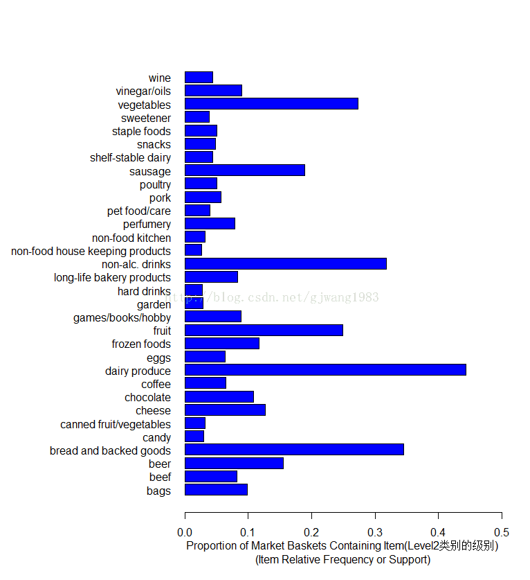
3 {dairy produce}

我們可以對比一下在aggregate前後的itemFrequency圖。

itemFrequencyPlot(Groceries, support = 0.025, cex.names=0.8, xlim = c(0,0.3),
  type = "relative", horiz = TRUE, col = "dark red", las = 1,
  xlab = paste("Proportion of Market Baskets Containing Item",
    "\n(Item Relative Frequency or Support)"))

horiz=TRUE: 讓柱狀圖水平顯示

cex.names=0.8:item的label（這個例子即縱軸）的大小乘以的係數。

las=1: 表示刻度的方向，1表示總是水平方向。

type="relative": 即support的值（百分比）。如果type=absolute表示顯示該item的count，而非support。預設就是relative。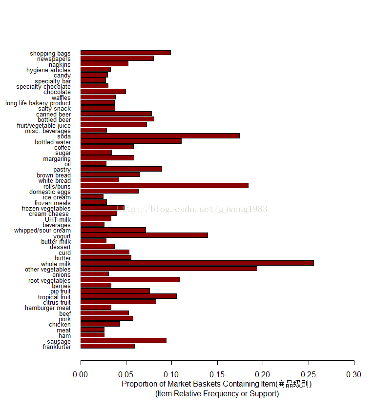

2. 規則的圖形展現

假設我們有這樣一個規則集合：

> second.rules <- apriori(groceries, 
+                         parameter = list(support = 0.025, confidence = 0.05))

Parameter specification:
 confidence minval smax arem  aval originalSupport support minlen maxlen target   ext
       0.05    0.1    1 none FALSE            TRUE   0.025      1     10  rules FALSE

Algorithmic control:
 filter tree heap memopt load sort verbose
    0.1 TRUE TRUE  FALSE TRUE    2    TRUE

apriori - find association rules with the apriori algorithm
version 4.21 (2004.05.09)        (c) 1996-2004   Christian Borgelt
set item appearances ...[0 item(s)] done [0.00s].
set transactions ...[55 item(s), 9835 transaction(s)] done [0.02s].
sorting and recoding items ... [32 item(s)] done [0.00s].
creating transaction tree ... done [0.00s].
checking subsets of size 1 2 3 4 done [0.00s].
writing ... [344 rule(s)] done [0.00s].
creating S4 object  ... done [0.00s].
> print(summary(second.rules))
set of 344 rules

rule length distribution (lhs + rhs):sizes
  1   2   3   4 
 21 162 129  32 

   Min. 1st Qu.  Median    Mean 3rd Qu.    Max. 
    1.0     2.0     2.0     2.5     3.0     4.0 

summary of quality measures:
    support          confidence           lift       
 Min.   :0.02542   Min.   :0.05043   Min.   :0.6669  
 1st Qu.:0.03030   1st Qu.:0.18202   1st Qu.:1.2498  
 Median :0.03854   Median :0.39522   Median :1.4770  
 Mean   :0.05276   Mean   :0.37658   Mean   :1.4831  
 3rd Qu.:0.05236   3rd Qu.:0.51271   3rd Qu.:1.7094  
 Max.   :0.44301   Max.   :0.79841   Max.   :2.4073  

mining info:
      data ntransactions support confidence
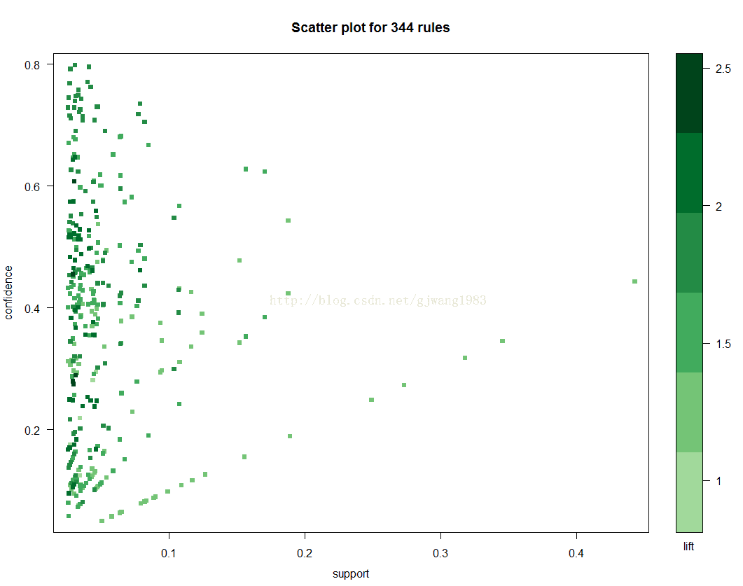
 groceries          9835   0.025       0.05

2.1 Scatter Plot

> plot(second.rules, 
+      control=list(jitter=2, col = rev(brewer.pal(9, "Greens")[4:9])),
+      shading = "lift")

shading = "lift"：表示在散點圖上顏色深淺的度量是lift。當然也可以設定為support 或者Confidence。

jitter=2：增加抖動值

col: 調色盤，預設是100個顏色的灰色調色盤。

brewer.pal(n, name): 建立調色盤：n表示該調色盤內總共有多少種顏色；name表示調色盤的名字（參考help）。

這裡使用Green這塊調色盤，引入9中顏色。

這幅散點圖表示了規則的分佈圖：大部分規則的support在0.1以內，Confidence在0-0.8內。每個點的顏色深淺代表了lift的值。

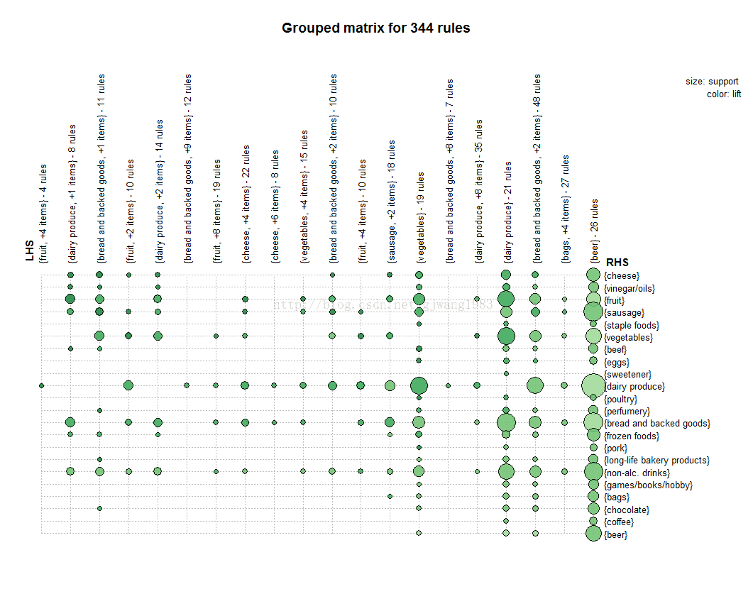
2.2 Grouped Matrix

> plot(second.rules, method="grouped",   
+      control=list(col = rev(brewer.pal(9, "Greens")[4:9])))

Grouped matrix-based visualization.

Antecedents (columns) in the matrix are grouped using clustering. Groups are represented as balloons in the matrix.

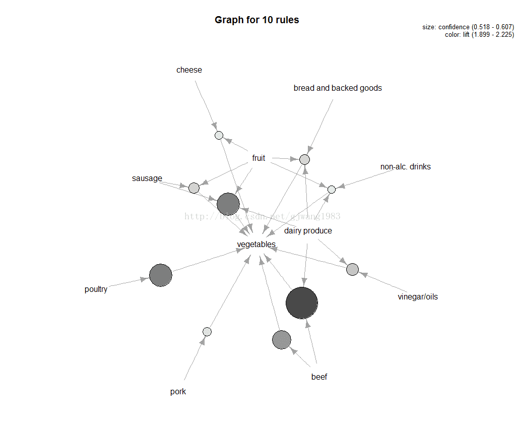
2.3 Graph

Represents the rules (or itemsets) as a graph

<strong>> plot(top.vegie.rules, measure="confidence", method="graph", 
+      control=list(type="items"), 
+      shading = "lift")</strong>

type=items表示每個圓點的入度的item的集合就是LHS的itemset

measure定義了圈圈大小，預設是support

顏色深淺有shading控制

關聯規則挖掘小結

1. 關聯規則是發現數據間的關係：可能會共同發生的那些屬性co-occurrence

2. 一個好的規則可以用lift或者FishersExact Test進行校驗。

3. 當屬性（商品）越多的時候，支援度會比較低。

4. 關聯規則的發掘是互動式的，需要不斷的檢查、優化。

FP-Growth

TO ADD Here

eclat

arules包中有一個eclat演算法的實現，用於發現頻繁項集。