CNN發展史：

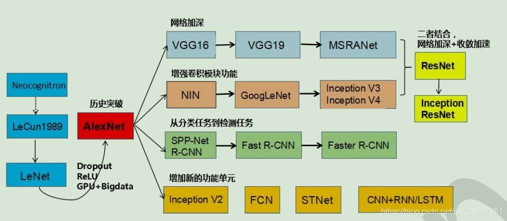
1.經典卷積神經網路

以下僅列出關於CNN的深層次理解：

卷積層

tensorflow中卷積層的建立函式：_conv1 = tf.nn.conv2d(_input_r, tf.Variable(tf.random_normal([3, 3, 1, 64], stddev=0.1)), strides=[1, 1, 1, 1], padding='SAME')  引數說明：

1. 輸入影象
2. tensor變數建立(正態分佈初始化(filter_height,fileter_width,in_channels,out_channels],方差))
3. stride=[1,stride,stride,1]
4. padding='SAME'or'VALID'(same是圈圈取零包裹)

1. 卷積核的通道數必須與輸入的一致，但可以有多個卷積核，如此輸出通道數便增多了
2. 經過卷積核之後的輸出影象大小：以高為例：  
3. 卷積核的意義，其實就跟影象處理當中的“影象分割”裡線檢測、邊緣檢測用的運算元一般：線檢測運算元--水平、+45°、-45°、垂直；邊緣檢測運算元：sobel、prewitt、Laplacian等，這些是基於影象的突變性和連續性，從“一階導數”、“二階導數”等數學原理所推匯出來的幾何特徵的提取運算元。而我們利用神經網路的BP反饋對卷積核進行訓練，則這個運算元則能夠幫助我們提取我們所需要的特徵。
4. 卷積核的分類--擴張卷積、轉置卷積、可分離卷積：http://www.sohu.com/a/159591827_390227
5. padding邊緣填充是為了不讓一些邊界消失，分為full、same、valid。
6. “區域性連線”--每個神經元（卷積層的一個畫素）僅與輸入神經元的一塊區域（輸入影象的一個區域性區域）連線，這塊區域性區域稱作感受野。如此保證了學習後的過濾器能夠對於區域性的輸入特徵有最強的響應。區域性連線的思想，也是受啟發於生物學裡面的視覺系統結構，視覺皮層的神經元就是區域性接受資訊的；而且區域性連線使得引數大量減少。
7. “權值共享”--計算同一個深度切片的神經元時採用的濾波器是共享的。共享權重在一定程度上講是有意義的，例如圖片的底層邊緣特徵與特徵在圖中的具體位置無關。但是在一些場景中是無意的，比如輸入的圖片是人臉，眼睛和頭髮位於不同的位置，希望在不同的位置學到不同的特徵 (參考斯坦福大學公開課)。請注意權重只是對於同一深度切片的神經元是共享的，在卷積層，通常採用多組卷積核提取不同特徵，即對應不同深度切片的特徵，不同深度切片的神經元權重是不共享，如此組成的特徵即為Feature map。另外，偏重對同一深度切片的所有神經元都是共享的。
8. “分散式表徵”--神經網路的重要性質，即如“編碼”一般，可將樣本從原始空間投影到一個更好的特徵空間中。

池化層

tensorflow中池化層的建立函式：_pool1 = tf.nn.max_pool(_conv1, ksize=[1, 2, 2, 1], strides=[1, 2, 2, 1], padding='SAME')

1. 池化層的作用：通過池化來降低卷積層輸出的特徵向量，同時改善結果（不易出現過擬合）。
2. 池化層的操作：max、mean。
3. “區域不變形”--pooling 這步綜合了局部特徵，失去了每個特徵的位置資訊。這很適合基於影象的任務，比如要判斷一幅圖裡有沒有貓這種生物，你可能不會去關心這隻貓出現在影象的哪個區域。但是在 NLP 裡，詞語在句子或是段落裡出現的位置，順序，都是很重要的資訊。

一個經典卷積神經網路的實現：input-conv1-relu-pooling1-conv2-relu-pooling2-dc1-output

n_input  = 784
n_output = 10
weights  = {
        'wc1': tf.Variable(tf.random_normal([3, 3, 1, 64], stddev=0.1)),
        'wc2': tf.Variable(tf.random_normal([3, 3, 64, 128], stddev=0.1)),
        'wd1': tf.Variable(tf.random_normal([7*7*128, 1024], stddev=0.1)),
        'wd2': tf.Variable(tf.random_normal([1024, n_output], stddev=0.1))
    }
biases   = {
        'bc1': tf.Variable(tf.random_normal([64], stddev=0.1)),
        'bc2': tf.Variable(tf.random_normal([128], stddev=0.1)),
        'bd1': tf.Variable(tf.random_normal([1024], stddev=0.1)),
        'bd2': tf.Variable(tf.random_normal([n_output], stddev=0.1))
    }

def conv_basic(_input, _w, _b, _keepratio):
        # INPUT
        _input_r = tf.reshape(_input, shape=[-1, 28, 28, 1])
        # CONV LAYER 1
        _conv1 = tf.nn.conv2d(_input_r, _w['wc1'], strides=[1, 1, 1, 1], padding='SAME')
        #_mean, _var = tf.nn.moments(_conv1, [0, 1, 2])
        #_conv1 = tf.nn.batch_normalization(_conv1, _mean, _var, 0, 1, 0.0001)
        _conv1 = tf.nn.relu(tf.nn.bias_add(_conv1, _b['bc1']))
        _pool1 = tf.nn.max_pool(_conv1, ksize=[1, 2, 2, 1], strides=[1, 2, 2, 1], padding='SAME')
        _pool_dr1 = tf.nn.dropout(_pool1, _keepratio)
        # CONV LAYER 2
        _conv2 = tf.nn.conv2d(_pool_dr1, _w['wc2'], strides=[1, 1, 1, 1], padding='SAME')
        #_mean, _var = tf.nn.moments(_conv2, [0, 1, 2])
        #_conv2 = tf.nn.batch_normalization(_conv2, _mean, _var, 0, 1, 0.0001)
        _conv2 = tf.nn.relu(tf.nn.bias_add(_conv2, _b['bc2']))
        _pool2 = tf.nn.max_pool(_conv2, ksize=[1, 2, 2, 1], strides=[1, 2, 2, 1], padding='SAME')
        _pool_dr2 = tf.nn.dropout(_pool2, _keepratio)
        # VECTORIZE
        _dense1 = tf.reshape(_pool_dr2, [-1, _w['wd1'].get_shape().as_list()[0]])
        # FULLY CONNECTED LAYER 1
        _fc1 = tf.nn.relu(tf.add(tf.matmul(_dense1, _w['wd1']), _b['bd1']))
        _fc_dr1 = tf.nn.dropout(_fc1, _keepratio)
        # FULLY CONNECTED LAYER 2
        _out = tf.add(tf.matmul(_fc_dr1, _w['wd2']), _b['bd2'])
        # RETURN
        out = { 'input_r': _input_r, 'conv1': _conv1, 'pool1': _pool1, 'pool1_dr1': _pool_dr1,
            'conv2': _conv2, 'pool2': _pool2, 'pool_dr2': _pool_dr2, 'dense1': _dense1,
            'fc1': _fc1, 'fc_dr1': _fc_dr1, 'out': _out
        }
        return out
print ("CNN READY")

x = tf.placeholder(tf.float32, [None, n_input])
y = tf.placeholder(tf.float32, [None, n_output])
keepratio = tf.placeholder(tf.float32)

# FUNCTIONS

_pred = conv_basic(x, weights, biases, keepratio)['out']
cost = tf.reduce_mean(tf.nn.softmax_cross_entropy_with_logits(labels=y, logits=_pred))
#使用了最先進的adam優化演算法，其中包含了正則化的思想，但不像傳統的正則化那樣。
optm = tf.train.AdamOptimizer(learning_rate=0.001).minimize(cost)
_corr = tf.equal(tf.argmax(_pred,1), tf.argmax(y,1)) 
accr = tf.reduce_mean(tf.cast(_corr, tf.float32)) 
init = tf.global_variables_initializer()
    
# SAVER
print ("GRAPH READY")

sess = tf.Session()
sess.run(init)

training_epochs = 30
batch_size      = 10
display_step    = 5
time1=time.time()
for epoch in range(training_epochs):
    avg_cost = 0.
    total_batch = int(mnist.train.num_examples/batch_size)
    #total_batch = 10
    # Loop over all batches
    for i in range(total_batch):
        batch_xs, batch_ys = mnist.train.next_batch(batch_size)
        # Fit training using batch data
        sess.run(optm, feed_dict={x: batch_xs, y: batch_ys, keepratio:0.7})
        # Compute average loss
        avg_cost += sess.run(cost, feed_dict={x: batch_xs, y: batch_ys, keepratio:1.})/total_batch

    # Display logs per epoch step
    if epoch % display_step == 0: 
        print ("Epoch: %03d/%03d cost: %.9f" % (epoch, training_epochs, avg_cost))
        train_acc = sess.run(accr, feed_dict={x: batch_xs, y: batch_ys, keepratio:1.})
        print (" Training accuracy: %.3f" % (train_acc))
        test_acc = sess.run(accr, feed_dict={x: testimg, y: testlabel, keepratio:1.})
        print (" Test accuracy: %.3f" % (test_acc))

print ("OPTIMIZATION FINISHED")
time_waste=time.time()-time1
print("The time wasting is:%dh %dm %ds"%(time_waste//(60*24),time_waste%(60*24)//60,time_waste%(60*24)%60))

Epoch: 000/030 cost: 0.122792258
 Training accuracy: 0.900
 Test accuracy: 0.986
Epoch: 005/030 cost: 0.012638518
 Training accuracy: 1.000
 Test accuracy: 0.993
Epoch: 010/030 cost: 0.006675720
 Training accuracy: 1.000
 Test accuracy: 0.992
Epoch: 015/030 cost: 0.005300980
 Training accuracy: 1.000
 Test accuracy: 0.992
Epoch: 020/030 cost: 0.003683299
 Training accuracy: 1.000
 Test accuracy: 0.990
Epoch: 025/030 cost: 0.003249645
 Training accuracy: 1.000
 Test accuracy: 0.993
OPTIMIZATION FINISHED
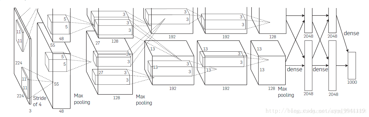
The time wasting is:0h 13m 54s

2.Alexnet

以上程式很多地方其實已經用到了Alexnet的特點了：像是RELU、dropout。

Alexnet的特點實際上就是：

1. 採用了三個連結層：2048、2048、1000
2. 啟用函式採用relu
3. 全連結層採用dropout
4. 在relu和pool之間採用區域性相應歸一化LRN，但是當net的層數到達11層時，這個lrn沒有作用，反而起了副作用；而且因為lrn在池化層前的計算會不經濟，所以後面的alexnet改進有把lrn放在了pool後面
5. conv-pool數更多了，達到5個
6. GPUS分散式計算，如圖所示
7. 擴充套件資料：隨機裁剪、旋轉......

LRN的介紹：

 引數可以百度LRN看看，這裡講講它的含義--來源於《深度學習與計算機視覺》

區域性相應歸一化模擬的是動物神經中的橫向抑制效應（將相似的記憶分開），從公式可以看出，如果在該位置，該通道和臨近通道的絕對值都比較大的話，歸一化之後值會有變得更小的趨勢。

3.模型的儲存和讀取

#儲存模型
saver = tf.train.Saver(max_to_keep=3)#最多儲存三個模型，再存入則會按照first delete
saver.save(sess, "save/nets/cnn_mnist_basic.ckpt-" + str(epoch))#將訓練好的計算圖存入該檔案

#讀取模型
epoch = training_epochs-1
saver.restore(sess, "save/nets/cnn_mnist_basic.ckpt-" + str(epoch))

test_acc = sess.run(accr, feed_dict={x: testimg, y: testlabel, keepratio:1.})
print (" TEST ACCURACY: %.3f" % (test_acc))

參考資料：https://github.com/scutan90/DeepLearning-500-questions