本文大部分內容翻譯自[Illustrated Self-Attention, Step-by-step guide to self-attention with illustrations and code](https://towardsdatascience.com/illustrated-self-attention-2d627e33b20a)，僅用於學習，如有翻譯不當之處，敬請諒解！ ### 什麼是Self-Attention（自注意力機制）？   如果你在想Self-Attention（自注意力機制）是否和Attention（注意力機制）相似，那麼答案是肯定的。它們本質上屬於同一個概念，擁有許多共同的數學運算。   一個Self-Attention模組擁有n個輸入，返回n個輸出。這麼模組裡面發生了什麼？從非專業角度看，Self-Attention（自注意力機制）允許輸入之間互相作用（“self”部分），尋找出誰更應該值得注意（“attention”部分）。輸出的結果是這些互相作用和注意力分數的聚合。 ### 一步步理解Self-Attention   理解分為以下幾步： 1. 準備輸入； 2. 初始化權重； 3. 獲取`key`，`query`和`value`； 4. 為第1個輸入計算注意力分數； 5. 計算softmax; 6. 將分數乘以values； 7. 對權重化後的values求和，得到輸出1； 8. 對其餘的輸入，重複第4-7步。 > 注意：實際上，這些數學運算都是向量化的，也就是說，所有的輸入都會一起經歷這些數學運算。我們將會在後面的程式碼部分看到。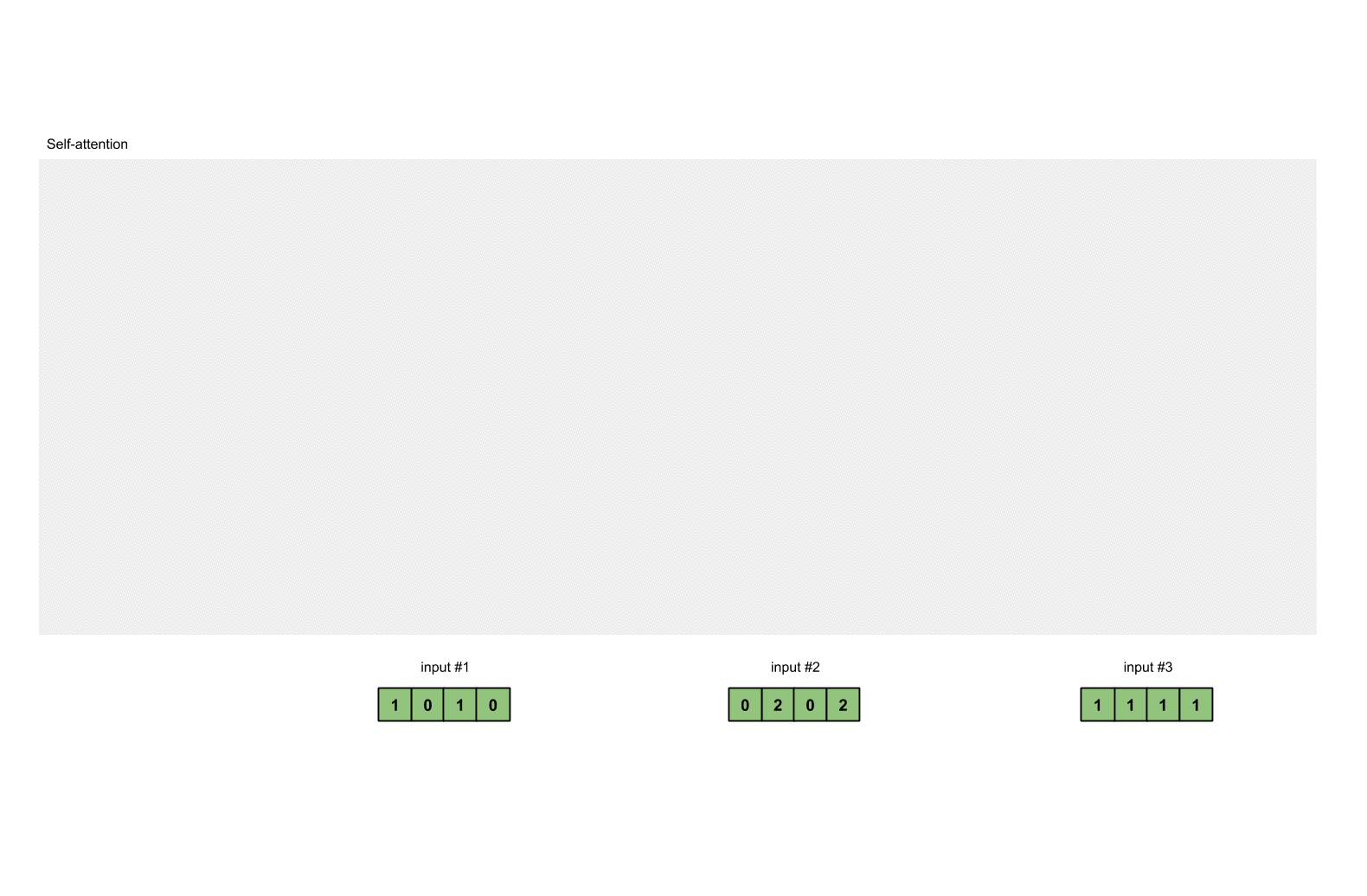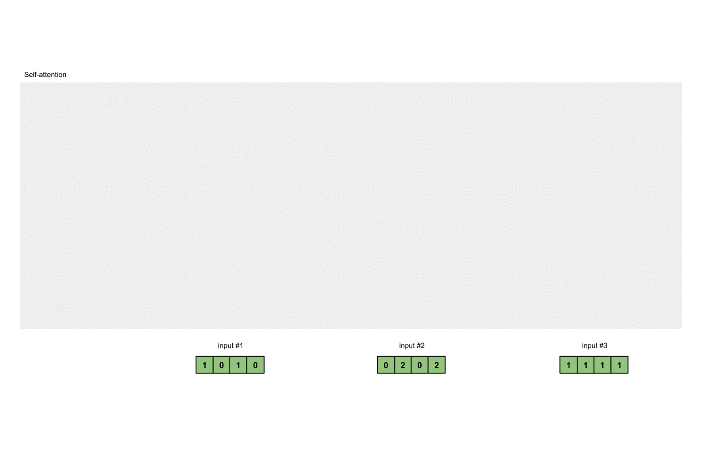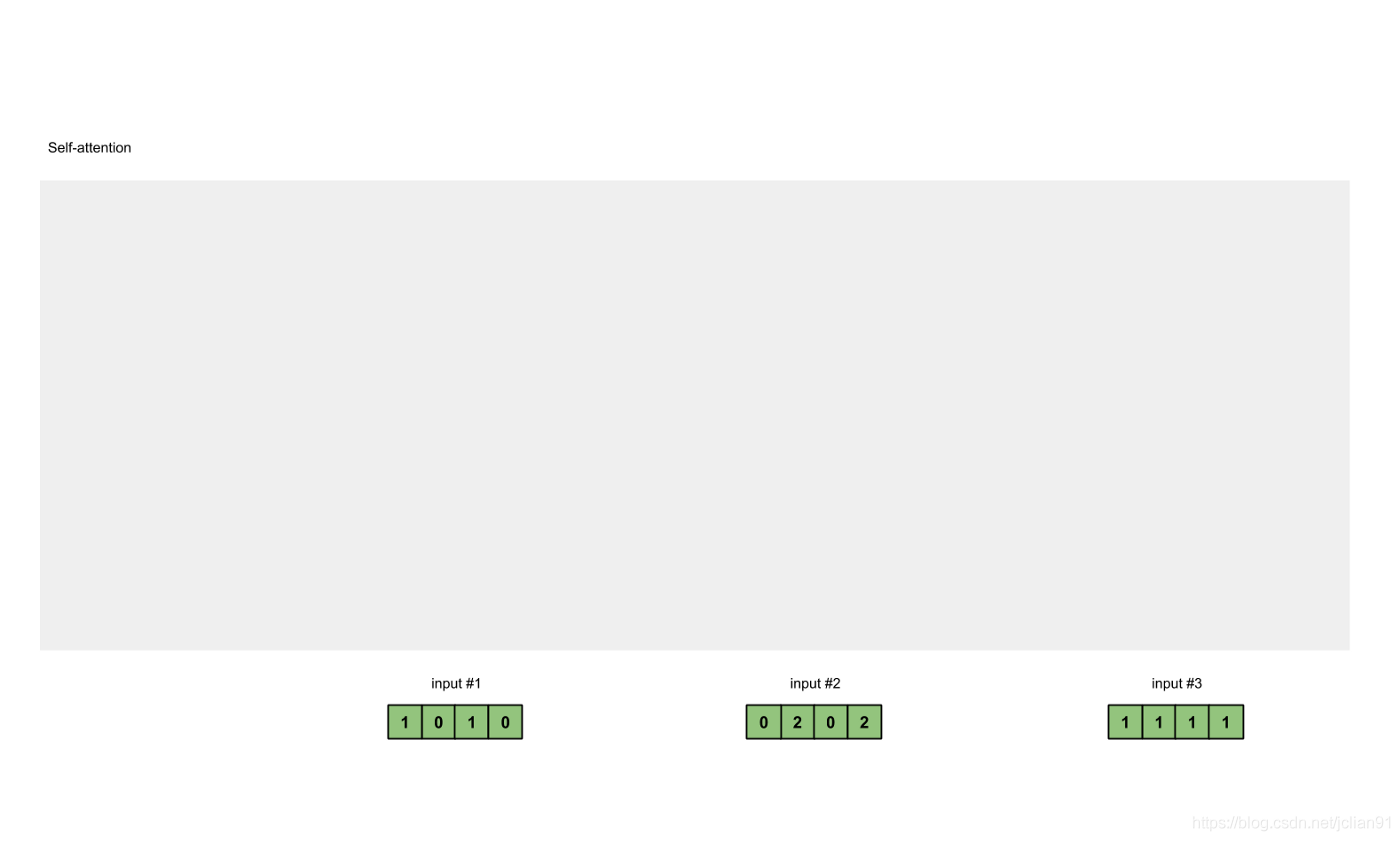 #### 第一步：準備輸入  在這個教程中，我們從3個輸入開始，每個輸入的維數為4。 ``` Input 1: [1, 0, 1, 0] Input 2: [0, 2, 0, 2] Input 3: [1, 1, 1, 1] ``` #### 第二步：初始化權重   每個輸入必須由三個表示（看下圖）。這些輸入被稱作`key`（橙色），`query`（紅色）`value`（紫色）。在這個例子中，我們假設我們想要的表示維數為3。因為每個輸入的維數為4，這就意味著每個權重的形狀為4×3。 >注意：我們稍後會看到`value`的維數也是output的維數。    為了獲取這些表示，每個輸入（綠色）會乘以一個權重的集合得到`keys`，乘以一個權重的集合得到`queries`，乘以一個權重的集合得到`values`。在我們的例子中，我們初始化三個權重的集合如下。   `key`的權重： ``` [[0, 0, 1], [1, 1, 0], [0, 1, 0], [1, 1, 0]] ```   `query`的權重： ``` [[1, 0, 1], [1, 0, 0], [0, 0, 1], [0, 1, 1]] ```   `value`的權重： ``` [[0, 2, 0], [0, 3, 0], [1, 0, 3], [1, 1, 0]] ``` > 注意： 在神經網路設定中，這些權重通常都是一些小的數字，利用隨機分佈，比如Gaussian, Xavier and Kaiming分佈，隨機初始化。在訓練開始前已經完成初始化。 ### 第三步：獲取`key`，`query`和`value`；   現在我們有了3個權重的集合，讓我們來給每個輸入獲取`key`，`query`和`value`。   第1個輸入的`key`表示： ``` [0, 0, 1] [1, 0, 1, 0] x [1, 1, 0] = [0, 1, 1] [0, 1, 0] [1, 1, 0] ```   利用相同的權重集合獲取第2個輸入的`key`表示： ``` [0, 0, 1] [0, 2, 0, 2] x [1, 1, 0] = [4, 4, 0] [0, 1, 0] [1, 1, 0] ```   利用相同的權重集合獲取第3個輸入的`key`表示： ``` [0, 0, 1] [1, 1, 1, 1] x [1, 1, 0] = [2, 3, 1] [0, 1, 0] [1, 1, 0] ```   更快的方式是將這些運算用向量來描述： ``` [0, 0, 1] [1, 0, 1, 0] [1, 1, 0] [0, 1, 1] [0, 2, 0, 2] x [0, 1, 0] = [4, 4, 0] [1, 1, 1, 1] [1, 1, 0] [2, 3, 1] ```    讓我們用相同的操作來獲取每個輸入的`value`表示：  最後是`query`的表示： ``` [1, 0, 1] [1, 0, 1, 0] [1, 0, 0] [1, 0, 2] [0, 2, 0, 2] x [0, 0, 1] = [2, 2, 2] [1, 1, 1, 1] [0, 1, 1] [2, 1, 3] ```  > 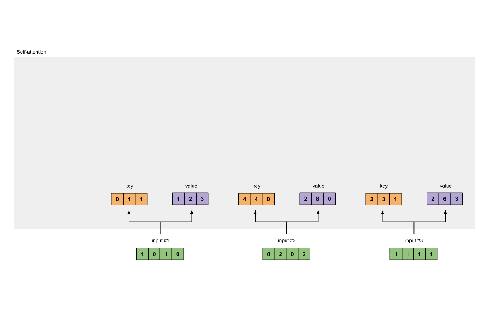注意：實際上，一個偏重向量也許會加到矩陣相乘後的結果。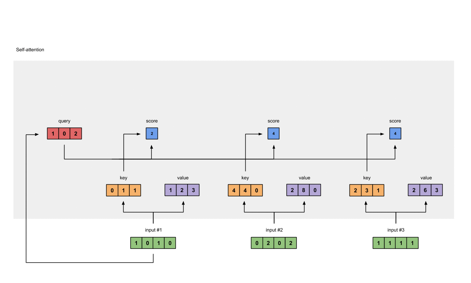 #### 第四步：為第1個輸入計算注意力分數    為了獲取注意力分數，我們從輸入1的`query`（紅色）和所有`keys`（橙色）的點積開始。因為有3個`key`表示（這是由於我們有3個輸入），我們得到3個注意力分數（藍色）。 ``` [0, 4, 2] [1, 0, 2] x [1, 4, 3] = [2, 4, 4] [1, 0, 1] ``` 注意到我們只用了輸入的`query`。後面我們會為其他的`queries`重複這些步驟。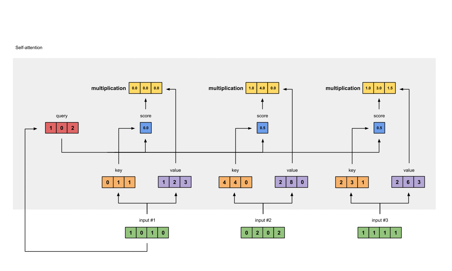 #### 第五步：計算softmax    對這些注意力分數進行softmax函式運算（藍色部分）。 ``` softmax([2, 4, 4]) = [0.0, 0.5, 0.5] ``` #### 第六步： 將分數乘以values    將每個輸入（綠色）的softmax作用後的注意力分數乘以各自對應的`value`（紫色）。這會產生3個向量（黃色）。在這個教程中，我們把它們稱作`權重化value`。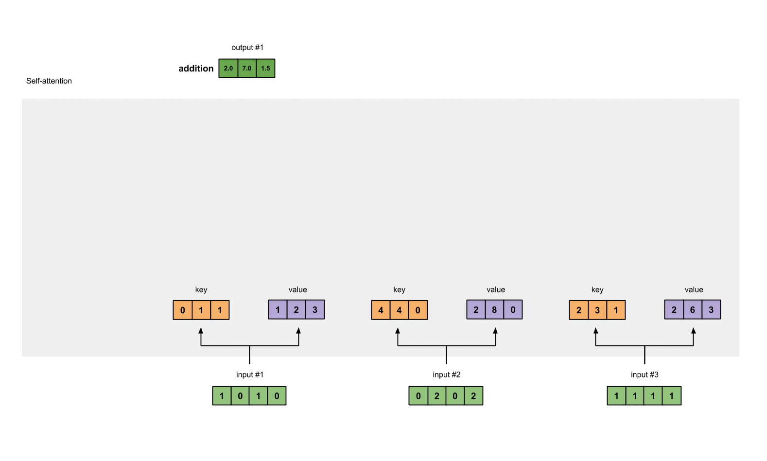 ``` 1: 0.0 * [1, 2, 3] = [0.0, 0.0, 0.0] 2: 0.5 * [2, 8, 0] = [1.0, 4.0, 0.0] 3: 0.5 * [2, 6, 3] = [1.0, 3.0, 1.5] ``` #### 第七步：對權重化後的values求和，得到輸出1    將`權重後value`按元素相加得到輸出1： ``` [0.0, 0.0, 0.0] + [1.0, 4.0, 0.0] + [1.0, 3.0, 1.5] ----------------- = [2.0, 7.0, 1.5] ```   產生的向量[2.0, 7.0, 1.5]（暗綠色）就是輸出1，這是基於輸入1的`query`表示與其它的`keys`，包括它自身的`key`互相作用的結果。 #### 第八步：對輸入2、3，重複第4-7步   既然我們已經完成了輸入1，我們重複步驟4-7能得到輸出2和3。這個可以留給讀者自己嘗試，相信聰明的你可以做出來。  ### 程式碼   這裡有PyTorch的實現程式碼，PyTorch是一個主流的Python深度學習框架。為了能夠很好地使用程式碼片段中的`@`運算子, `.T` and `None`操作，請確保Python≥3.6，PyTorch ≥1.3.1。 #### 1. 準備輸入 ```python import torch x = [ [1, 0, 1, 0], # Input 1 [0, 2, 0, 2], # Input 2 [1, 1, 1, 1] # Input 3 ] x = torch.tensor(x, dtype=torch.float32) ``` #### 2. 初始化權重 ```python w_key = [ [0, 0, 1], [1, 1, 0], [0, 1, 0], [1, 1, 0] ] w_query = [ [1, 0, 1], [1, 0, 0], [0, 0, 1], [0, 1, 1] ] w_value = [ [0, 2, 0], [0, 3, 0], [1, 0, 3], [1, 1, 0] ] w_key = torch.tensor(w_key, dtype=torch.float32) w_query = torch.tensor(w_query, dtype=torch.float32) w_value = torch.tensor(w_value, dtype=torch.float32) ``` #### 3. 獲取`key`，`query`和`value` ```python keys = x @ w_key querys = x @ w_query values = x @ w_value print(keys) # tensor([[0., 1., 1.], # [4., 4., 0.], # [2., 3., 1.]]) print(querys) # tensor([[1., 0., 2.], # [2., 2., 2.], # [2., 1., 3.]]) print(values) # tensor([[1., 2., 3.], # [2., 8., 0.], # [2., 6., 3.]]) ``` #### 4. 為第1個輸入計算注意力分數 ``` attn_scores = querys @ keys.T # tensor([[ 2., 4., 4.], # attention scores from Query 1 # [ 4., 16., 12.], # attention scores from Query 2 # [ 4., 12., 10.]]) # attention scores from Query 3 ``` #### 5. 計算softmax ```python from torch.nn.functional import softmax attn_scores_softmax = softmax(attn_scores, dim=-1) # tensor([[6.3379e-02, 4.6831e-01, 4.6831e-01], # [6.0337e-06, 9.8201e-01, 1.7986e-02], # [2.9539e-04, 8.8054e-01, 1.1917e-01]]) # For readability, approximate the above as follows attn_scores_softmax = [ [0.0, 0.5, 0.5], [0.0, 1.0, 0.0], [0.0, 0.9, 0.1] ] attn_scores_softmax = torch.tensor(attn_scores_softmax) ``` #### 6. 將分數乘以values ```python weighted_values = values[:,None] * attn_scores_softmax.T[:,:,None] # tensor([[[0.0000, 0.0000, 0.0000], # [0.0000, 0.0000, 0.0000], # [0.0000, 0.0000, 0.0000]], # # [[1.0000, 4.0000, 0.0000], # [2.0000, 8.0000, 0.0000], # [1.8000, 7.2000, 0.0000]], # # [[1.0000, 3.0000, 1.5000], # [0.0000, 0.0000, 0.0000], # [0.2000, 0.6000, 0.3000]]]) ``` #### 7. 對權重化後的values求和，得到輸出 ``` outputs = weighted_values.sum(dim=0) # tensor([[2.0000, 7.0000, 1.5000], # Output 1 # [2.0000, 8.0000, 0.0000], # Output 2 # [2.0000, 7.8000, 0.3000]]) # Output 3 ``` > 注意：PyTorch已經提供了這個API，名字為`nn.MultiheadAttention`。但是，這個API需要你提供PyTorch的Tensor形式的key，value，query。還有，這個模組的輸出會經歷一個線性變換。 ### 自己實現？   以下是筆者自己寫的部分。   對於不熟悉PyTorch的讀者來說，上述的向量操作理解起來有點困難，因此，筆者自己用簡單的Python程式碼實現了一遍上述Self-Attention的過程。   完整的Python程式碼如下： ```python # -*- coding: utf-8 -*- from typing import List import math from pprint import pprint x = [[1, 0, 1, 0], # Input 1 [0, 2, 0, 2], # Input 2 [1, 1, 1, 1] # Input 3 ] w_key = [[0, 0, 1], [1, 1, 0], [0, 1, 0], [1, 1, 0] ] w_query = [[1, 0, 1], [1, 0, 0], [0, 0, 1], [0, 1, 1] ] w_value = [[0, 2, 0], [0, 3, 0], [1, 0, 3], [1, 1, 0] ] # vector dot of two vectors def vector_dot(list1: List[float or int], list2: List[float or int]) -> float or int: dot_sum = 0 for element_i, element_j in zip(list1, list2): dot_sum += element_i * element_j return dot_sum # get weights matrix by x, using matrix multiplication def get_weights_matrix_by_x(x, weight_matrix): x_matrix = [] for i in range(len(x)): x_row = [] for j in range(len(weight_matrix[0])): x_row.append(vector_dot(x[i], [_[j] for _ in weight_matrix])) x_matrix.append(x_row) return x_matrix # softmax function def softmax(x: List[float or int]) -> List[float or int]: x_sum = sum([math.exp(_) for _ in x]) return [math.exp(_)/x_sum for _ in x] x_key = get_weights_matrix_by_x(x, w_key) x_value = get_weights_matrix_by_x(x, w_value) x_query = get_weights_matrix_by_x(x, w_query) # print(x_key) # print(x_value) # print(x_query) outputs = [] for query in x_query: score_list = [vector_dot(query, key) for key in x_key] softmax_score_list = softmax(score_list) weights_list = [] for i in range(len(softmax_score_list)): weights = [softmax_score_list[i] * _ for _ in x_value[i]] weights_list.append(weights) output = [] for j in range(len(weights_list[0])): output.append(sum([_[j] for _ in weights_list])) outputs.append(output) pprint(outputs) ``` 輸出結果如下： ``` [[1.9366210616669624, 6.683105308334811, 1.5950684074995565], [1.9999939663351456, 7.9639915951322156, 0.0539764053125496], [1.9997046127769653, 7.759892254657784, 0.3583892946751152]] ``` ### 總結   本文主要講述瞭如何一步一步來實現Self-Attention機制，對於想要自己實現演算法的讀者來說，值得一讀。   本文分享到此結束，感謝大家