這篇文章將講解如何使用python建立多層神經網路。在閱讀這篇文章之前，建議先閱讀上一篇文章:理解神經網路，從簡單的例子開始。講解的是單層的神經網路。如果你已經閱讀了上一篇文章，你會發現這篇文章的程式碼和上一篇基本相同，理解起來也相對容易。

上一篇文章使用了9行程式碼編寫一個單層的神經網路。而現在，問題變得更加複雜了。下面是訓練輸入資料和訓練輸出資料，如果輸入資料是[1，1，0]，最後的結果是什麼呢？

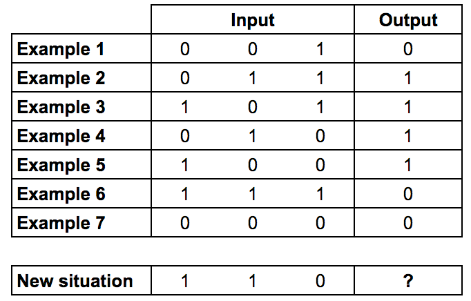
從上面的輸入輸出資料可以找出規律：第一和第二列的值“異或”之後得到output的值，而第三列沒有關係。所謂的異或，就是相同為0，相異為1.
所以，當輸入資料為[1，1，0]時，結果為0。
但是，這個在單層網路節點中是很難實現的，因為input和output之間沒有一對一的對應關係。所以，可以考慮使用多層的神經網路，或者說增加一個隱藏層，叫layer1，它能夠處理input的合併問題。

從圖中可以看出，第1層的輸出進入第2層。現在神經網路能夠處理第一層的輸出資料和第二層（也就是最終輸出的資料集）之間的關係。隨著神經網路學習，它將通過調整兩層的權重來放大這些相關性。

實際上，影象識別和這個很相似。比如下面圖片中，一個畫素和蘋果沒有直接的關係，但是許多畫素組合在一起就能夠構成一個蘋果的樣子，也就產生了關係。

這裡通過增加更多層神經來處理“組合”問題，便是所謂的深度學習了。下面是多層神經網路的python程式碼。解釋會在程式碼註釋中和程式碼後面。

from numpy import exp, array, random, dot


class NeuronLayer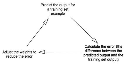
 
():
    def __init__(self, number_of_neurons, number_of_inputs_per_neuron):
        self.synaptic_weights = 2 * random.random((number_of_inputs_per_neuron, number_of_neurons)) - 1


class NeuralNetwork():
    def __init__(self, layer1, layer2):
        self.layer1 = layer1
        self.layer2 = layer2

    # The Sigmoid function, which describes an S shaped curve.
 

    # We pass the weighted sum of the inputs through this function to
    # normalise them between 0 and 1.
    def __sigmoid(self, x):
        return 1 / (1 + exp(-x))

    # The derivative of the Sigmoid function.
    # This is the gradient of the Sigmoid curve.
    # It indicates how confident we are about the existing weight.
    def __sigmoid_derivative(self, x):
        return x * (1 - x)

    # We train the neural network through a process of trial and error.
    # Adjusting the synaptic weights each time.
    def train(self, training_set_inputs, training_set_outputs, number_of_training_iterations):
        for iteration in range(number_of_training_iterations):
            # Pass the training set through our neural network
            output_from_layer_1, output_from_layer_2 = self.think(training_set_inputs)

            # Calculate the error for layer 2 (The difference between the desired output
            # and the predicted output).
            layer2_error = training_set_outputs - output_from_layer_2
            layer2_delta = layer2_error * self.__sigmoid_derivative(output_from_layer_2)

            # Calculate the error for layer 1 (By looking at the weights in layer 1,
            # we can determine by how much layer 1 contributed to the error in layer 2).
            layer1_error = layer2_delta.dot(self.layer2.synaptic_weights.T)
            layer1_delta = layer1_error * self.__sigmoid_derivative(output_from_layer_1)

            # Calculate how much to adjust the weights by
            layer1_adjustment = training_set_inputs.T.dot(layer1_delta)
            layer2_adjustment = output_from_layer_1.T.dot(layer2_delta)

            # Adjust the weights.
            self.layer1.synaptic_weights += layer1_adjustment
            self.layer2.synaptic_weights += layer2_adjustment

    # The neural network thinks.
    def think(self, inputs):
        output_from_layer1 = self.__sigmoid(dot(inputs, self.layer1.synaptic_weights))
        output_from_layer2 = self.__sigmoid(dot(output_from_layer1, self.layer2.synaptic_weights))
        return output_from_layer1, output_from_layer2

    # The neural network prints its weights
    def print_weights(self):
        print( "    Layer 1 (4 neurons, each with 3 inputs): ")
        print( self.layer1.synaptic_weights)
        print( "    Layer 2 (1 neuron, with 4 inputs):")
        print( self.layer2.synaptic_weights)

if __name__ == "__main__":

    #Seed the random number generator
    random.seed(1)

    # Create layer 1 (4 neurons, each with 3 inputs)
    layer1 = NeuronLayer(4, 3)

    # Create layer 2 (a single neuron with 4 inputs)
    layer2 = NeuronLayer(1, 4)

    # Combine the layers to create a neural network
    neural_network = NeuralNetwork(layer1, layer2)

    print ("Stage 1) Random starting synaptic weights: ")
    neural_network.print_weights()

    # The training set. We have 7 examples, each consisting of 3 input values
    # and 1 output value.
    training_set_inputs = array([[0, 0, 1], [0, 1, 1], [1, 0, 1], [0, 1, 0], [1, 0, 0], [1, 1, 1], [0, 0, 0]])
    training_set_outputs = array([[0, 1, 1, 1, 1, 0, 0]]).T

    # Train the neural network using the training set.
    # Do it 60,000 times and make small adjustments each time.
    neural_network.train(training_set_inputs, training_set_outputs, 60000)

    print ("Stage 2) New synaptic weights after training: ")
    neural_network.print_weights()

    # Test the neural network with a new situation.
    print ("Stage 3) Considering a new situation [1, 1, 0] -> ?: ")
    hidden_state, output = neural_network.think(array([1, 1, 0]))
    print (output)

上圖是深度學習的計算週期

和上篇部落格中的單層神經網路相比，這裡是多層，也就是增加了隱藏層。當神經網路計算第二層的error誤差值的時候，會把這個error向後面一層也即是第一次傳播，從而計算並調整第一層節點的權值。也就是，第一層的error誤差值是從上一層也即是第二層所傳播回來的值中計算得到的，這樣就能夠知道第一層對第二層的誤差有多大的貢獻。

執行上面的程式碼，會得到下面所示的結果。

Stage 1) Random starting synaptic weights: 
    Layer 1 (4 neurons, each with 3 inputs): 
[[-0.16595599  0.44064899 -0.99977125 -0.39533485]
 [-0.70648822 -0.81532281 -0.62747958 -0.30887855]
 [-0.20646505  0.07763347 -0.16161097  0.370439  ]]
    Layer 2 (1 neuron, with 4 inputs):
[[-0.5910955 ]
 [ 0.75623487]
 [-0.94522481]
 [ 0.34093502]]
Stage 2) New synaptic weights after training: 
    Layer 1 (4 neurons, each with 3 inputs): 
[[ 0.3122465   4.57704063 -6.15329916 -8.75834924]
 [ 0.19676933 -8.74975548 -6.1638187   4.40720501]
 [-0.03327074 -0.58272995  0.08319184 -0.39787635]]
    Layer 2 (1 neuron, with 4 inputs):
[[ -8.18850925]
 [ 10.13210706]
 [-21.33532796]
 [  9.90935111]]
Stage 3) Considering a new situation [1, 1, 0] -> ?: 
[ 0.0078876]

這篇文章是本人根據這篇部落格寫的。一定程度上算是在做翻譯的工作。本人特別推薦該原始碼的風格，一看就知道這是程式設計經驗豐富之人才能寫出來的程式碼，清晰明瞭，看起來特別舒服。

結束！ 轉載請標明出處，感謝！