
Python機器學習(二) Logistic迴歸建模分類例項——信用卡欺詐監測(上)
Logistic迴歸建模分類例項——信用卡欺詐監測
現有一個creditcard.csv(點此下載)資料集,其中包含不同客戶信用卡的特徵資料(V1、V2……V28、Amount)和標籤資料(Class),利用Logistic迴歸建模,通過這個模型預測客戶信用卡是否有被欺詐的風險。
import numpy as
- 1
- 2
- 3
- 4
- 5
- 6
- 7
- 8
- 9
- 10
- 11
- 12
- 13
% matplotlib inline表示將圖表嵌入到Notebook中。如果不加這一行程式碼,下面的圖2中的柱狀圖會顯示不出來。
將creditcard.csv中的資料讀到data中,因為creditcard.csv中的資料中Amount這一列比較特殊,其他列都在(-1,1)的區間內,而Amount這一兩列浮動範圍比較的,要知道特徵資料的浮動範圍越大,在建模過程中對於預測結果的影響就越大,但就這組資料來說我們並有足夠的先驗資訊來說明特徵資料的重要程度,故我們要對所有特徵資料一視同仁,讓他們都在(-1,1)之間。所以我們要對資料進行一些預處理,首先就要通過sklearn.preprocessing中的StandardScaler模組將Amount這一列的資料進行歸一化(標準化)操作。而後資料中有一列是Time,這一列資料是無用的,也就是說對於信用卡欺詐預測是沒有用的,所以我們要將其刪掉。
注意:data.drop([‘Amount’,’Time’], axis=1) 不會改變data本身,所以要將其賦值給data。筆者在用的時候以為它和reverse(),sort()這些函式一樣會改變資料本身,在這兒踩了一腳坑。
data[‘Amount’].values.reshape(-1,1)中reshape後(-1,1)表示將這個陣列變換成X*1的形式,至於X是多少就要看原始陣列中到底有多少元素了。
因為一般情況下,我們得到的原始資料集中都是不能直接拿來用的,它們要麼有大量無用資訊,要麼有缺失資料……,總之對於原始資料的預處理是必不可少的。下面就是通過data.head()顯示出來的處理完成的資料預覽圖。 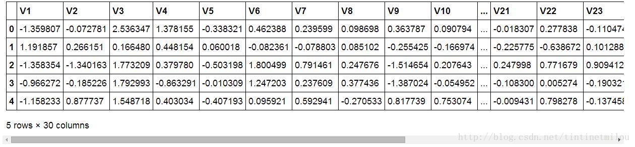
count_classes = pd.value_counts(data['Class'], sort = True).sort_index()print count_classescount_classes.plot(kind = 'bar')plt.title("Fraud class histogram")plt.xlabel("Class")plt.ylabel("Frequency")
- 1
- 2
- 3
- 4
- 5
- 6
通過matplotlib.pyplot來畫一個圖,統計一下資料中正負樣本的個數,結果如下圖所示:
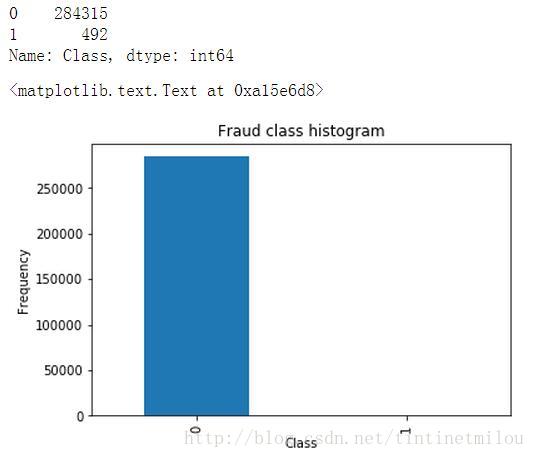
由圖可知,我們的資料中的負樣本(本例中1表示信用卡有被欺詐風險,為負樣本)是很少的,這叫做樣本不均衡,如果我們不進行處理,直接用這樣的資料來進行訓練建模,那得到的結果是很糟糕的(有多糟糕見下文)。所以我們要進行樣本資料處理,這用兩種方法:下采樣和過取樣。本篇部落格主要介紹下采樣的實現步驟,下一篇介紹過取樣。
下采樣
就是從數量比較多的那類樣本中,隨機選出和與數量比較少的那類樣本數量相同的樣本,最終組成正負樣本數量相同的樣本集進行訓練建模。
X = data.ix[:,data.columns != 'Class']Y = data.ix[:,data.columns == 'Class']number_record_fraud = len(Y[Y.Class==1])fraud_indices = np.array(data[data.Class == 1].index)normal_indices = np.array(data[data.Class == 0].index)random_normal_indices = np.array(np.random.choice(normal_indices,number_record_fraud,replace=False))under_sample_indices = np.concatenate([fraud_indices,random_normal_indices])under_sample_data = data.iloc[under_sample_indices,:]X_under_sample = under_sample_data.ix[:,under_sample_data.columns != 'Class']Y_under_sample = under_sample_data.ix[:,under_sample_data.columns == 'Class']from sklearn.cross_validation import train_test_splitX_train_under_sample,X_test_under_sample,Y_train_under_sample,Y_test_under_sample = train_test_split(X_under_sample,Y_under_sample,test_size=0.3,random_state=0)X_train, X_test, Y_train, Y_test = train_test_split(X, Y, test_size=0.3, random_state=0)
- 1
- 2
- 3
- 4
- 5
- 6
- 7
- 8
- 9
- 10
- 11
- 12
- 13
- 14
- 15
- 16
- 17
- 18
- 19
- 20
通過np.random.choice在正樣本的索引(normal_indices)中隨機選負樣本個數(number_record_fraud )個索引。
np.concatenate將負樣本和挑選的負樣本索引進行合併成
根據上面得到的索引來去原始資料中提取特徵(X_under_sample)和標籤(Y_under_sample )
接下來是用klearn.cross_validation 模組中的train_test_split來將上面提取到的資料(特徵,標籤)分為訓練集和測試集,測試佔總體的30%。X_train, X_test, Y_train, Y_test是對原始未進行下采樣的資料進行的同樣操作得到的,這些資料後面測試的時候會用到。
交叉驗證
機器學習中,當將要採用的機器學習演算法確定後,模型訓練的實質就是確定一系列的引數了(調參)。調參其實就是各種試,但也是有章可循的。首先要用一些資料和某個引數來訓練得到一個模型,然後用另外一些資料來帶入剛才訓練好的模型,輸出結果和標籤進行比較,計算出來一個評價指標,根據這個評價指標來判斷剛才帶入的那個引數到底好不好。
先說上面的評價指標,最常見的評價指標為精度:
可見recall只和TP和FN有關係,那當FP很大時(本來為0,沒有欺詐風險,但預測為1,預測成有風險),所以在調參的時候不僅要看recall值,還要通過混淆矩陣,看看FP這個值。
上面是用下采樣處理得到的測試資料來求recall和混淆矩陣的,因為下采樣得到的資料相比於原始資料是很少的,所以這個測試結果沒什麼說服力,所以我們要用原始資料(沒有經過下采樣的資料)來進行測試。
lr = LogisticRegression(C = best_c, penalty = 'l1')lr.fit(X_train_under_sample,Y_train_under_sample.values.ravel())Y_pred = lr.predict(X_test.values)# Compute confusion matrixcnf_matrix = confusion_matrix(Y_test,Y_pred)np.set_printoptions(precision=2)print("Recall metric in the testing dataset: ", float(cnf_matrix[1,1])/(cnf_matrix[1,0]+cnf_matrix[1,1]))# Plot non-normalized confusion matrixclass_names = [0,1]plt.figure()plot_confusion_matrix(cnf_matrix , classes=class_names , title='Confusion matrix')plt.show()
- 1
- 2
- 3
- 4
- 5
- 6
- 7
- 8
- 9
- 10
- 11
- 12
- 13
- 14
- 15
- 16
- 17
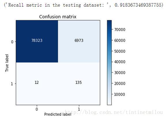
由上圖可知,通過下采樣處理資料得到的邏輯迴歸模型,雖然recall值挺高的,但NP值非常高,也就是誤殺率非常高。這也是用下采樣處理資料的一個弊端吧,如果採用過取樣來處理資料,效果就會好很多。
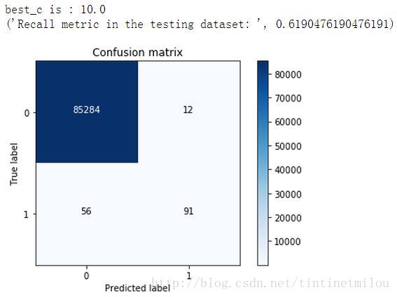
前面說樣本不均衡,如果不進行處理,直接用這樣的資料來進行訓練建模,那得到的結果是很糟糕,現在就看看到底有多糟糕。
best_c = printing_Kfold_scores(X_train,Y_train)lr = LogisticRegression(C = best_c, penalty = 'l1')lr.fit(X_train,Y_train.values.ravel())Y_pred = lr.predict(X_test.values)# Compute confusion matrixcnf_matrix = confusion_matrix(Y_test,Y_pred)np.set_printoptions(precision=2)print("Recall metric in the testing dataset: ", float(cnf_matrix[1,1])/(cnf_matrix[1,0]+cnf_matrix[1,1]))# Plot non-normalized confusion matrixclass_names = [0,1]plt.figure()plot_confusion_matrix(cnf_matrix , classes=class_names , title='Confusion matrix')plt.show()
- 1
- 2
- 3
- 4
- 5
- 6
- 7
- 8
- 9
- 10
- 11
- 12
- 13
- 14
- 15
- 16
- 17
- 18
邏輯迴歸模型中除了懲罰力度引數C需要整定,Threshold也可以調調,預設不做處理相當於Threshold為0.5
lr = LogisticRegression(C = 0.01, penalty = 'l1')lr.fit(X_train_under_sample,Y_train_under_sample.values.ravel())y_pred_undersample_proba = lr.predict_proba(X_test_under_sample.values)thresholds = [0.1,0.2,0.3,0.4,0.5,0.6,0.7,0.8,0.9]plt.figure(figsize=(10,10))recall_accs = []j = 1for i in thresholds: y_test_predictions_high_recall = y_pred_undersample_proba[:,1] > i plt.subplot(3,3,j) j += 1 # Compute confusion matrix cnf_matrix = confusion_matrix(Y_test_under_sample,y_test_predictions_high_recall) np.set_printoptions(precision=2) recall_acc = float(cnf_matrix[1,1])/(cnf_matrix[1,0]+cnf_matrix[1,1]) print'Threshold>=%s Recall: '%i, recall_acc recall_accs.append(recall_acc) # Plot non-normalized confusion matrix class_names = [0,1] plot_confusion_matrix(cnf_matrix , classes=class_names , title='Threshold>=%s'%i)
- 1
- 2
- 3
- 4
- 5
- 6
- 7
- 8
- 9
- 10
- 11
- 12
- 13
- 14
- 15
- 16
- 17
- 18
- 19
- 20
- 21
- 22
- 23
- 24
- 25
- 26
- 27
- 28
- 29
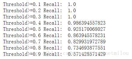
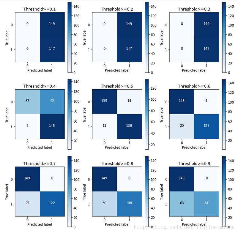
由上圖看Threshold還是為0.5是較好。
再分享一下我老師大神的人工智慧教程吧。零基礎!通俗易懂!風趣幽默!還帶黃段子!希望你也加入到我們人工智慧的隊伍中來!https://blog.csdn.net/jiangjunshow