如何繪製caffe網路訓練曲線
阿新 • • 發佈:2019-01-08
當我們設計好網路結構後,在神經網路訓練的過程中,迭代輸出的log資訊中,一般包括,迭代次數,訓練損失代價,測試損失代價,測試精度等。本文提供一段示例,簡單講述如何繪製訓練曲線(training curve)。
首先看一段訓練的log輸出,網路結構引數的那段忽略,直接跳到訓練迭代階段:
I0627 21:30:06.004370 15558 solver.cpp:242] Iteration 0, loss = 21.6953
I0627 21:30:06.004420 15558 solver.cpp:258] Train net output #0: loss = 21.6953 (* 1 = 21.6953 loss) 這是一個普通的網路訓練輸出,含有1個loss,可以看出solver.prototxt的部分引數為:
test_interval: 2000
base_lr: 0.01
lr_policy: "step" # or "multistep"
gamma: 0.96
display: 100
stepsize: 50000 # if is "multistep", the first stepvalue is set as 50000
snapshot_prefix: "train_net/net"
當然,上面的分析,即便不理會,對下面的程式碼也沒什麼影響,繪製訓練曲線本質就是檔案操作,從上面的log檔案中,我們可以看出:
- 對於每個出現欄位
] Iteration和loss =的文字行,含有訓練的迭代次數以及損失代價; - 對於每個含有欄位
] Iteration和Testing net (#0)的文字行,含有測試的對應的訓練迭代次數; - 對於每個含有欄位
#2:和loss/top-5的文字行,含有測試top-5的精度。
根據這些分析,就可以對文字進行如下處理:
import os
import sys
import numpy as np
import matplotlib.pyplot as plt
import math
import re
import pylab
from pylab import figure, show, legend
from mpl_toolkits.axes_grid1 import host_subplot

# read the log file
fp = open('log.txt', 'r')

train_iterations = []
train_loss = []
test_iterations = []
test_accuracy = []

for ln in fp:
  # get train_iterations and train_loss
  if '] Iteration ' in ln and 'loss = ' in ln:
    arr = re.findall(r'ion \b\d+\b,',ln)
    train_iterations.append(int(arr[0].strip(',')[4:]))
    train_loss.append(float(ln.strip().split(' = ')[-1]))
  # get test_iteraitions
  if '] Iteration' in ln and 'Testing net (#0)' in ln:
    arr = re.findall(r'ion \b\d+\b,',ln)
    test_iterations.append(int(arr[0].strip(',')[4:]))
  # get test_accuracy
  if '#2:' in ln and 'loss/top-5' in ln:
    test_accuracy.append(float(ln.strip().split(' = ')[-1]))

fp.close()

host = host_subplot(111)
plt.subplots_adjust(right=0.8) # ajust the right boundary of the plot window
par1 = host.twinx()
# set labels
host.set_xlabel("iterations")
host.set_ylabel("log loss")
par1.set_ylabel("validation accuracy")

# plot curves
p1, = host.plot(train_iterations, train_loss, label="training log loss")
p2, = par1.plot(test_iterations, test_accuracy, label="validation accuracy")

# set location of the legend,
# 1->rightup corner, 2->leftup corner, 3->leftdown corner
# 4->rightdown corner, 5->rightmid ...
host.legend(loc=5)

# set label color
host.axis["left"].label.set_color(p1.get_color())
par1.axis["right"].label.set_color(p2.get_color())
# set the range of x axis of host and y axis of par1
host.set_xlim([-1500, 160000])
par1.set_ylim([0., 1.05])

plt.draw()
plt.show()
示例程式碼中,添加了簡單的註釋,如果網路訓練的log輸出與本中所列出的不同,只需要略微修改其中的一些引數設定,就能繪製出訓練曲線圖。
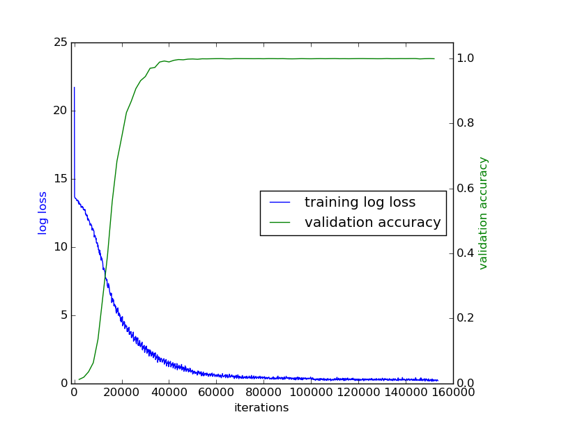
最後附上繪製出的訓練曲線圖: