LogisticRegression原理及演算法

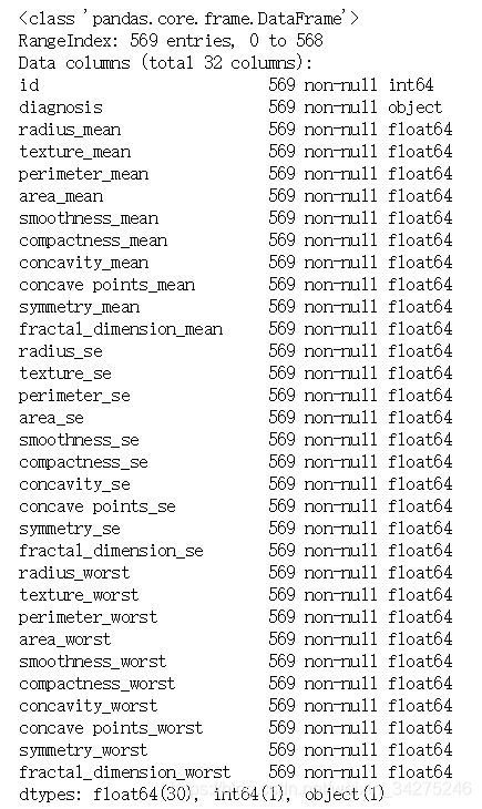
該資料共有569個樣本，每個樣本有11列不同的數值：第一列是檢索的ID，中間9列是與腫瘤相關的醫學特徵，以及一列表徵腫瘤型別的數值。所有9列用於表示腫瘤醫學特質的數值均被量化為1-10之間的數字。

import pandas as pd
import numpy as np
import matplotlib.pyplot as plt

data = pd.read_csv(r'D:\machinelearningDatasets\BreastCancerLR\Breast cancer.csv')

data.head()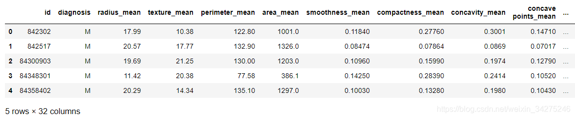
 

data.info()
#data.isnull().any().sum()
#plt.matshow(data.corr())

提取特徵和標籤資料：

y = data.iloc[:,1] 是錯誤的，這其實沒有標題，序號也沒有！列索引即使一列也要用範圍提取。

x = data.iloc[:,2:31]
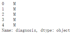
y = data.iloc[:,1:2]

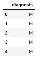
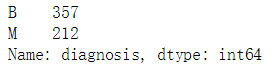
檢視診斷結果中良性和惡性腫瘤個數：

y.diagnosis.value_counts()

劃分資料集：

from sklearn.model_selection import train_test_split
x_train,
 
 x_test, y_train, y_test = train_test_split(x, y, test_size=0.2, random_state=10)

y = y.values.ravel()

使用交叉驗證優化演算法：

from sklearn.model_selection import cross_val_predict
from sklearn.model_selection import cross_val_score

from sklearn.linear_model import LogisticRegression

for i in ['l1','l2'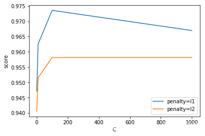
 
]:
    lgrlist = []
    for j in [1,10,100,1000]:
        lgr = LogisticRegression(C=j, penalty=i)
        lgr_cv_score = cross_val_score(lgr,x_train,y_train,cv=5)
        lgr_cv_score_meanscore = lgr_cv_score.mean()
        lgrlist.append(lgr_cv_score_meanscore)
    plt.plot([1,10,100,1000], lgrlist, label='penalty='+str(i))
    plt.legend()
plt.xlabel('C')
plt.ylabel('score')

lgr = LogisticRegression(C=100, penalty='l1')
lgr_cv_score = cross_val_score(lgr, x_train, y_train, cv=5)
lgr_meanscore = lgr_cv_score.mean()

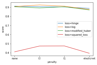
隨機梯度下降分類演算法：

sklearn.linear_model.SGDClassifier

from sklearn.linear_model import SGDClassifier

for i in ['hinge', 'log', 'modified_huber','squared_loss']:
    SGDClist = []
    for j in ['none','l2','l1','elasticnet']:
        SGDC = SGDClassifier(penalty=j, loss=i, max_iter=1000)
        SGDC_cv_score = cross_val_score(SGDC,x_train,y_train,cv=5)
        SGDC_cv_score_meanscore = SGDC_cv_score.mean()
        SGDClist.append(SGDC_cv_score_meanscore)
    plt.plot(['none','l2','l1','elasticnet'], SGDClist, label='loss='+str(i))
    plt.legend()
plt.xlabel('penalty')
plt.ylabel('score')

SGDC = SGDClassifier(loss='log', penalty='l2', max_iter=1000)
SGDC_cv_score = cross_val_score(SGDC, x_train, y_train, cv=5)
SGDC_meanscore = SGDC_cv_score.mean()

評估分類演算法：

evaluating=pd.DataFrame({'lr':lr_cv_test_score,'SGDC':SGDC_cv_test_score})
evaluating

evaluating.plot.kde()

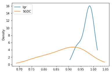
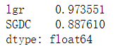
evaluating.mean().sort_values(ascending=False)

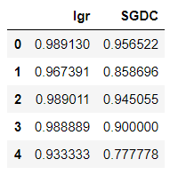
在測試集上驗證模型效能：

#lgr
lgr.fit(x_train,y_train)
lgr_y_predict_score = lgr.score(x_test, y_test)

#SGDC
SGDC.fit(x_train,y_train)
SGDC_y_predict_score = SGDC.score(x_test, y_test)

predict_score = {
        'lgr':lgr_y_predict_score,
        'SGDC':SGDC_y_predict_score
        }
predict_score = pd.DataFrame(predict_score, index=['score']).transpose()
predict_score.sort_values(by='score',ascending = False)

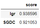
可見邏輯迴歸分類比隨機梯度下降分類表現更好。

繪製學習曲線：

import sys
sys.path.append(r'C:\Users\Qiuyi\Desktop\scikit-learn code\code\common')
from utils import plot_learning_curve
from sklearn.model_selection import ShuffleSplit
title = 'Learning Curves (logisticRegression)'
cv = ShuffleSplit(n_splits=10, test_size=0.25, random_state=0)
plot_learning_curve(plt,lgr,title,x,y,ylim=(0.7, 1.01), cv=cv, n_jobs=4)

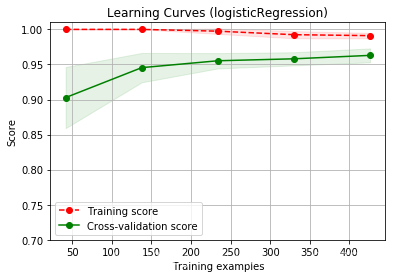
訓練樣本評分高，交叉驗證樣本評分也高，但兩評分之間間隙還比較大，可以採用更多的資料來訓練模型。