
機器學習實踐 學習筆記2 Classifying with k-Nearest Neighbors
k-近鄰演算法(k-Nearest Neighbors,kNN)
工作原理:
knn演算法屬於監督型別演算法。首先我們有樣本訓練集,知道每一條資料的分類。繼而,我們輸入沒有分類的新資料,將新資料的每個特徵與樣本集中的對應項進行比較,提取樣本集中最相思的資料,這樣我們可以獲得該資料的分類。一般來說,我們只選擇樣本集中前k個最相似的資料,通常k不大於20.最後,選擇k個相似資料中出現最多的分類,作為新資料的分類,此為k近鄰演算法。
優點:
精度高,對異常數值不敏感,無資料輸入假定。
缺點:計算複雜度高,空間複雜度高。無法給出任何資料的基礎結構資訊,因此我們也無法知曉平均
例項樣本和典型例項樣本具有什麼特徵
適用資料範圍:數值型,標稱型(numeric values,nominal values)
虛擬碼:
(1)計算樣本資料集中的點與當前帶分類資料的點之間的距離(計算相似程度)
(2)按照距離遞增排序
(3)選取與當前距離最小的前K個點
(4)確定k個點所在類別的出現頻率
(5)返回出現頻率最高的類別作為預測分類
python程式碼:
def createDataSet():#建立樣本訓練集
	group = array([[1.0,1.1],[1.0,1.0],[0,0],[0,0.1]])
	labels = ['A','A','B','B']
	return group,labels
#intX:待分類資料(向量),dataSet,labels:樣本訓練集,k def classi0(intX, dataSet, labels, k): dataSetSize = dataSet.shape[0]#訓練集大小 diffMat = tile(intX,(dataSetSize,1)) - dataSet#把待分類資料向量複製成與訓練集等階,對應項求差 sqDiffMat = diffMat**2#各項平方 sqDistances = sqDiffMat.sum(axis=1)#axis=1,將一個矩陣的每一行向量相加 distances = sqDistances**0.5#開方,求出距離 sortedDistIndicies = distances.argsort()#從小到大排序,返回陣列的索引 classCount = {} for i in range(k):#遍歷前K個樣本訓練集 voteILabel = labels[sortedDistIndicies[i]]#對應分類 classCount[voteILabel] = classCount.get(voteILabel,0) + 1#計數 sortedClassCount = sorted(classCount.iteritems(),key=operator.itemgetter(1),reverse=True)#排序 return sortedClassCount[0][0]#返回統計最多的分類
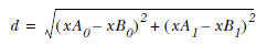
其中,距離的計算使用了歐式幾何:
測試分類器:
錯誤率是常用的檢驗分類器的方法:
通過大量已知分類的測試資料,計算出分類器給出錯誤答案的次數除以測試的總次數。
準備資料:python獲取文字資料:
409208.3269760.953952largeDoses
144887.1534691.673904smallDoses
260521.4418710.805124didntLike
假設文字資料儲存在datingTestSet.txt文字中
def file2matrix(filename):
    fr = open(filename)
    arrayOLines = fr.readlines()#獲取所有資料,以行為單位切割
    numberOfLines = len(arrayOLines)
    returnMat = zeros((numberOfLines,3))#構建矩陣,以0填充
    classLabelVector = []
    index = 0
    for line in arrayOLines:
        line = line.strip()
        listFromLine = line.split('\t')#以tab分割為陣列
        returnMat[index,:] = listFromLine[0:3]#copy資料
        classLabelVector.append(listFromLine[-1])#儲存對應的分類
        index += 1
    return returnMat,classLabelVector
分析資料:
使用Matplotlib建立散點圖分析資料:
import matplotlib
import matplotlib.pyplot as plt
fig = plt.figure()
ax = fig.add_subplot(111)#add_subplot(mnp)新增子軸、圖。subplot(m,n,p)或者subplot(mnp)此函式最常用:subplot是將多個圖畫到一個平面上的工具。其中,m表示是圖排成m行,n表示圖排成n列,也就是整個figure中有n個圖是排成一行的,一共m行,如果第一個數字是2就是表示2行圖。p是指你現在要把曲線畫到figure中哪個圖上,最後一個如果是1表示是從左到右第一個位置。
ax.scatter(datingDataMat[:,1], datingDataMat[:,2],15.0*array(map(int,datingLabels)),15.0*array(map(int,datingLabels)))#以第二列和第三列為x,y軸畫出雜湊點,給予不同的顏色和大小
#scatter(x,y,s=1,c="g",marker="s",linewidths=0)
#s:雜湊點的大小,c:雜湊點的顏色,marker:形狀,linewidths:邊框寬度
plt.show()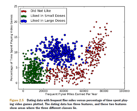
準備資料:
歸一化資料值
為了減少特徵值之間因度量不同帶來權重的偏差,需要將資料歸一化。所謂的歸一化,是講數值範圍處理在0~1或-1~1之間。
可以用如下公式:
newValue = (oldValue-min)/(max-min)
max和min分別是該項資料集特徵中的最大值和最小值。
據此可寫出歸一化函式
def autoNorm(dataSet):
    minVals = dataSet.min(0)#一維陣列,值為各項特徵(列)中的最小值
    maxVals = dataSet.max(0)
    ranges = maxVals - minVals
    normDataSet = zeros(shape(dataSet))
    m = dataSet.shape[0]
    normDataSet = dataSet - tile(minVals, (m,1))
    normDataSet = normDataSet/tile(ranges, (m,1))
    return normDataSet, ranges, minVals
測試演算法:
通常只用90%的資料來訓練分類器,剩餘資料去測試分類器,獲取正確/錯誤率。
def datingClassTest():
    hoRatio = 0.10
    datingDataMat,datingLabels = file2matrix('datingTestSet.txt')
    normMat, ranges, minVals = autoNorm(datingDataMat)
    m = normMat.shape[0]
    numTestVecs = int(m*hoRatio)
    errorCount = 0.0
    for i in range(numTestVecs):
        classifierResult = classi0(normMat[i,:],normMat[numTestVecs:m,:],datingLabels[numTestVecs:m],3)
        print "the classifier came back with: %s, the real answer is: %s" %  (classifierResult, datingLabels[i])
        if (classifierResult != datingLabels[i]): errorCount += 1.0
    print "the total error rate is: %f" % (errorCount/float(numTestVecs))
例項:數字識別系統
(1)收集資料
提供文字的文字檔案,大小都為32*32,每個數字大概有200個樣本
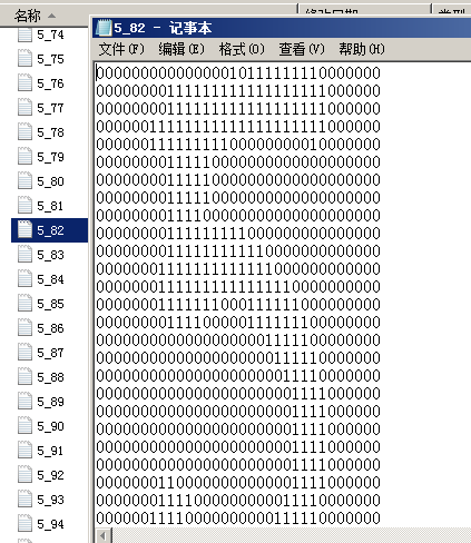
(2)準備資料,把資料轉換為上文中分類器可用的一維vector向量,從32*32變為1*24
def img2vector(filename):
	returnVect = zeros((1,1024))
	fr = open(filename)
	for i in range(32):
	lineStr = fr.readline()
	for j in range(32):
		returnVect[0,32*i+j] = int(lineStr[j])
	return returnVect
(3)測試演算法
def handwritingClassTest():
	hwLabels = []
	trainingFileList = listdir('trainingDigits')#樣本資料
	m = len(trainingFileList)
	trainingMat = zeros((m,1024))
	for i in range(m):
		fileNameStr = trainingFileList[i]
		fileStr = fileNameStr.split('.')[0]
		classNumStr = int(fileStr.split('_')[0])
		hwLabels.append(classNumStr)
		trainingMat[i,:] = img2vector('trainingDigits/%s' % fileNameStr)
	testFileList = listdir('testDigits')#測試資料
	errorCount = 0.0
	mTest = len(testFileList)
	for i in range(mTest):
		fileNameStr = testFileList[i]
		fileStr = fileNameStr.split('.')[0]
		classNumStr = int(fileStr.split('_')[0])
		vectorUnderTest = img2vector('testDigits/%s' % fileNameStr)
		classifierResult = classify0(vectorUnderTest, trainingMat, hwLabels, 3)
		print "the classifier came back with: %d, the real answer is: %d" % (classifierResult, classNumStr)
		if (classifierResult != classNumStr): errorCount += 1.0
	print "\nthe total number of errors is: %d" % errorCount
	print "\nthe total error rate is: %f" % (errorCount/float(mTest))