
如何用LaTeX寫公式(示例了十餘個公式,涵蓋了大多情況)
阿新 • • 發佈:2018-12-29
版權宣告:本文為博主原創文章轉載請標明地址:
https://mp.csdn.net/postedit/84580272
SSIM(structural similarity index),即結構相似性,公式如下:
![]()
接下來我就講一講怎麼寫這個公式:
1.首先, 用公式用\begin{equation} 和 \end{equation}作為開頭和結尾,這樣會產生公式並標註(1)序號,
2.分數:用要用 \frac{分子}{分母}
3.希臘字母表

4.上標下標
上標用^下標用_

還有集合等更多參見https://blog.csdn.net/young951023/article/details/79601664
5.括號
可以使用 \left 和 \right 來顯示不同的括號:

6.求和
\sum
7.乘號和點乘
乘號: \times
點乘: \cdot
一些示例:
示例一(SSIM):
\begin{equation}
SSIM(x,y)=\frac{\left(2\mu_x\mu_y+c1\right)\left(\sigma_{xy}+c2\right)}
{\left(\mu_x^2+\mu_y^2+c1\right)\left(\sigma_x^2+\sigma_y^2+c2\right)}
\end{equation}

Where $\mu_x$ is the average of x, $\mu_y$ is the average of y, $\sigma_x^2$ is the variance of x, $\sigma_y^2$ is the variance of y, and $\sigma_{xy}$ is the covariance of x and y. C1=(k1L)2, C1=(k1L)2, is a constant used to maintain stability. L is the dynamic range of the pixel value. K1 = 0.01, k2 = 0.03. The structural similarity ranges from 0 to 1. When the two images are identical, the value of SSIM is equal to one.
執行結果:

示例二:
\[ \int \!\!\! \int \!\!\! \int_V
\left| \psi(\mathbf{r},t) \right|^2\,dx\,dy\,dz\]
represents the probability that the particle is to be found
within the region~$V$ at time~$t$
執行結果:

示例三:
$\psi(\mathbf{r},t)$ of a particle satisfies the
\emph{Schr\"{o}dinger Wave Equation}
\[ i\hbar\frac{\partial \psi}{\partial t}
= \frac{-\hbar^2}{2m} \left(
\frac{\partial^2}{\partial x^2}
+ \frac{\partial^2}{\partial y^2}
+ \frac{\partial^2}{\partial z^2}
\right) \psi + V \psi.\]
執行結果:

示例四:
\begin{equation}

\hat{y} = \mathop{\argmax}_{y \in GEN(x)}{\mathbf{w} \cdot \Phi(x, y)}

\end{equation}
執行結果:

在用 argmax 和 argmin 要匯入包:
\usepackage{amsmath}
\usepackage{amssymb}
\DeclareMathOperator*{\argmax}{argmax}
示例五:
Image Signature(I_i) = sign(DCT2(I_i))執行結果:

示例六:
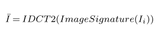
\bar{I}=IDCT2(Image Signature(I_i))執行結果:
示例七:
R=g\ast (\bar{I}\circ \bar{I})執行結果:

示例八:
\begin{equation}
M=\frac{\sum_{i\in \Omega }\cdot S}{\sum_{i\in \Omega }\cdot 1}
\end{equation}
where $\Omega$ is a non-salient area with its saliency value $R<0.6$; $S$ means the saturation graph of the non-salient regions.
執行結果:

示例九:
S(x,y)=\left\{
\begin{matrix}
\frac{U(x,y)-V(x,y)}{U(x,y)} & \quad \quad if\quad U(x,y)\neq 0\\
0 & otherwise
\end{matrix}
\right.
執行結果:

示例十:
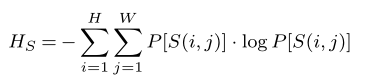
\begin{equation}
H_{S}=-\sum_{i=1}^{H}\sum_{j=1}^{W}{P}[S(i,j)]\cdot\log{P}[S(i,j)]
\label{func:02}
\end{equation}
執行結果:
示例11:
\begin{equation}
Q_{v}=\exp \left [ (H_{S}-u)/d -\exp \left ( (H_{s}-u)/d \right )\right ]/d
\end{equation}執行結果:![]()
示例12:
Q=\frac{Q_{v}\cdot{M}}{\sqrt{\min(Q_v,M)}}.執行結果:

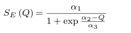
示例13:
\begin{equation}
S_{E}\left ( Q \right )=\frac{\alpha _{1}}{1+\exp \frac{\alpha_{2}-Q}{\alpha_{3}}}
\end{equation}
執行結果:
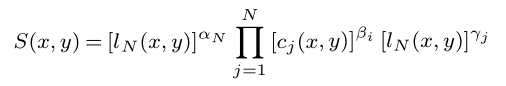
示例14:
S(x,y)=\left[l_N(x,y)\right]^{\alpha_N}\prod_{j=1}^{N}\left[c_j(x,y)\right]^{\beta_i}\left[l_N(x,y)\right]^{\gamma_j}執行結果:
參考文獻:
https://blog.csdn.net/xxzhangx/article/details/52778539
http://blog.sina.com.cn/s/blog_5e16f1770100fs38.html