How to use APIs with Pandas and store the results in Redshift

Here is an easy tutorial to help understand how you can use Pandas to get data from a RESTFUL API and store into a database in AWS Redshift.

Some basic understanding of Python (with Requests, Pandas and JSON libraries), REST APIs, Jupyter Notebook, AWS S3 and Redshift would be useful.

The goal of the tutorial is to use the geographical coordinates (longitude and latitude) provided in a CSV file to call an external API and reverse geocode the coordinates (i.e. get location details) and lastly store the response data in a Redshift table. Please note you may require caching approval from the API data supplier.

We will load the CSV with Pandas, use the Requests library to call the API, store the response into a Pandas Series and then a CSV, upload it to a S3 Bucket and copy the final data into a Redshift Table.The steps mentioned above are by no means the only way to approach this and the task can be performed by many different ways.

The dataset we will use contains country population as measured by the World Bank in 2013 and can be found on the below website.

Let’s begin.

Step 1 — Download the dataset

Links to column explanation and dataset

The first thing is to download the CSV file from the above website.

Step 2 — Start Jupyter Notebook and load the dataset into memory with Python

Install Jupyter Notebook (with Anaconda or otherwise) and fire it up by typing the following commands in the terminal while in the directory you wish to save the notebook.

Assuming you have installed the required libraries let’s load the CSV file into memory.

import pandas as pdimport requestsimport jsonimport timefrom pandas.io.json import json_normalize df = pd.read_csv('Global_country_populations_2013.csv') df = df[['CountryName','lat','lon']]df.head()

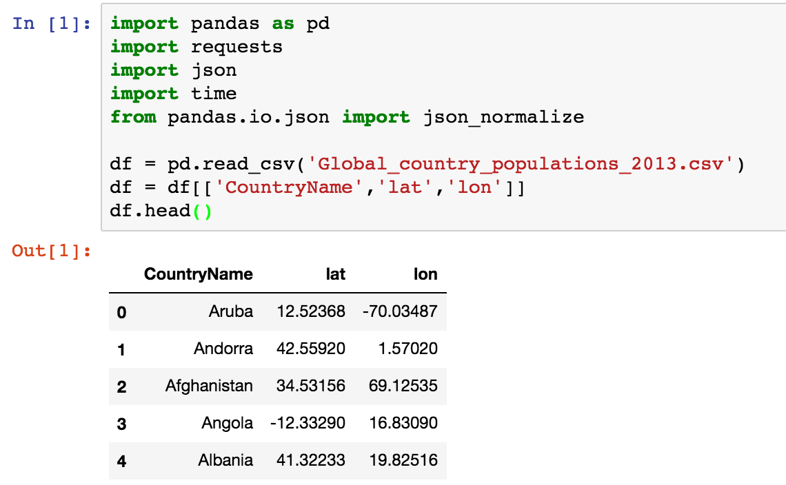
We have also imported other libraries as we will need them later on. The ‘read_csv()’ method will read your CSV file into a Pandas DataFrame. Please note you need to specify the path to file here if its not stored in the same directory. We then truncate the DataFrame to keep only the columns we need mainly [“CountryName”, “lat”, “lon”].

Step 3 — Define function to call API

The API we will use for the reverse geocoding is LocationIQ (from Unwired Labs) which offers free non commercial use with a rate of 60 calls/min and 10,000 calls per day.

def get_reverse_geocode_data(row):    try:        YOUR_API_KEY = 'xxxxxxxxxxx'        url = 'https://eu1.locationiq.org/v1/reverse.php?key=' + YOUR_API_KEY + '&lat=' + str(row['lat']) + '&lon=' + str(row['lon']) + '&format=json'                response = (requests.get(url).text)        response_json = json.loads(response)        time.sleep(0.5)        return response_json        except Exception as e:        raise e

In the above code we have defined a function — get_reverse_geocode_data(row). Once you sign up, you will get an API key which you need to include here along with the endpoint or URL and required parameters which you can obtain from the documentation. The parameter ‘row’ refers to each row of columns ‘lat’ and ‘lon’ of the Pandas DataFrame that will be passed as input to the API. The Requests library is used to make a HTTPS GET request to the url and receive the response using the ‘.text’ method.

You can use ‘json.loads()’ to convert the response from a JSON string into a JSON object which is easy to work with. The ‘time.sleep(0.5)’ parameter is used to control the calls to the API due to limitations set by the free tier plan (60 calls per min). For commercial high volume plans this won’t be necessary.

Step 4 — Call the function using the DataFrame Columns as parameters

df['API_response'] = df.apply(get_reverse_geocode_data,axis=1)df['API_response'].head()

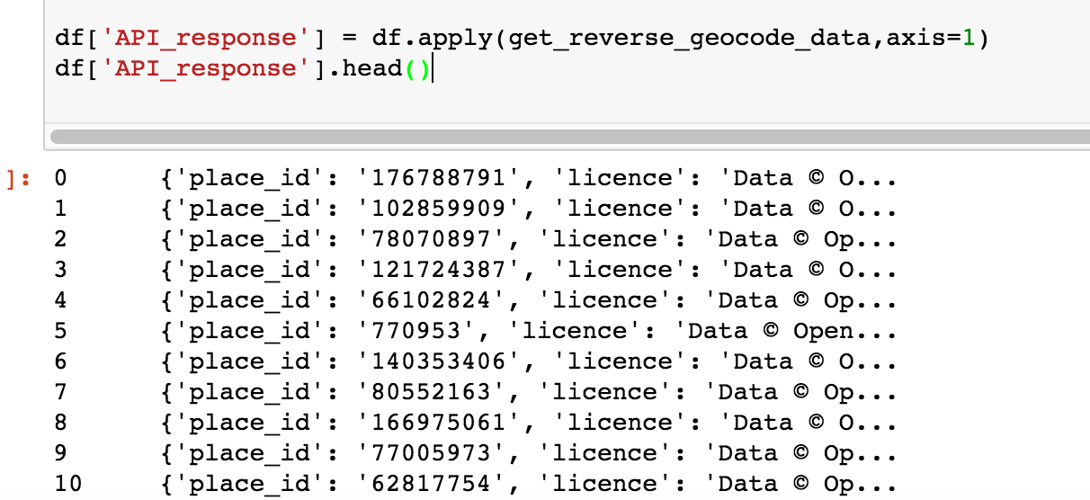
You can use the ‘df.apply()’ method to apply the function to the entire DataFrame. The ‘axis=1’ parameter is used to apply the function across the columns. The ‘row’ parameter we used earlier enables us to reference any column of the DataFrame we wish to use as input and takes the column value at that row as input for that particular execution.

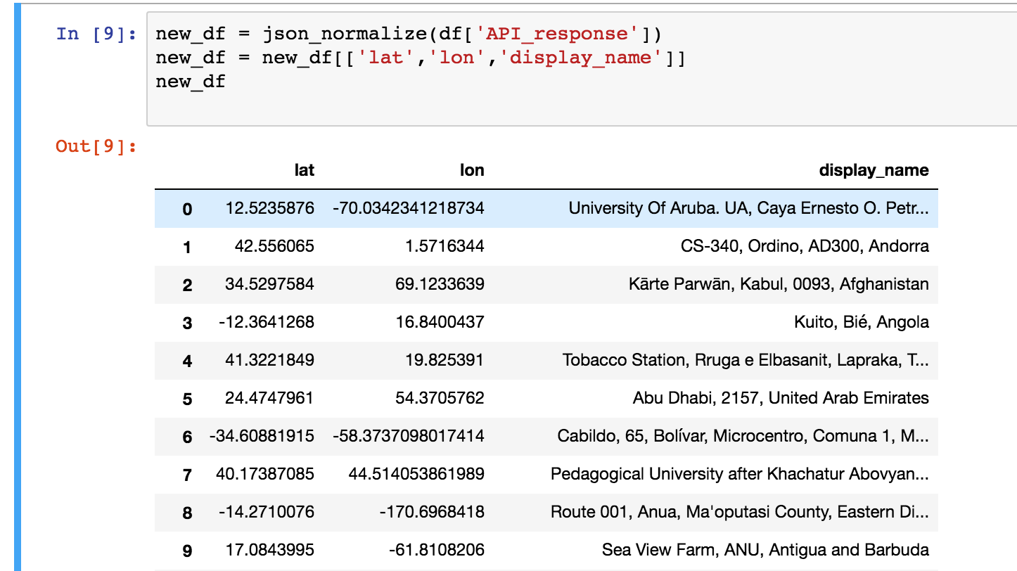
Step 5 — Normalise or Flatten the JSON response

Now that you have successfully received the JSON response from the API, its time to flatten it into columns and pick out the fields you wish to keep.

new_df = json_normalize(df['API_response'])new_df = new_df[['lat','lon','display_name']]new_df

The ‘json_normalize()’ function is great for this. You can pass in the Pandas Series you wish to normalize as argument and it returns a new Pandas DataFrame with the columns flattened. You can then join this new DataFrame to your old one by using the Foreign Key or in this case we will only use the new DataFrame. Let’s only keep the ‘display_name’ field (from the API_response) along with ‘lat’ and ‘lon’. Below is the new DataFrame

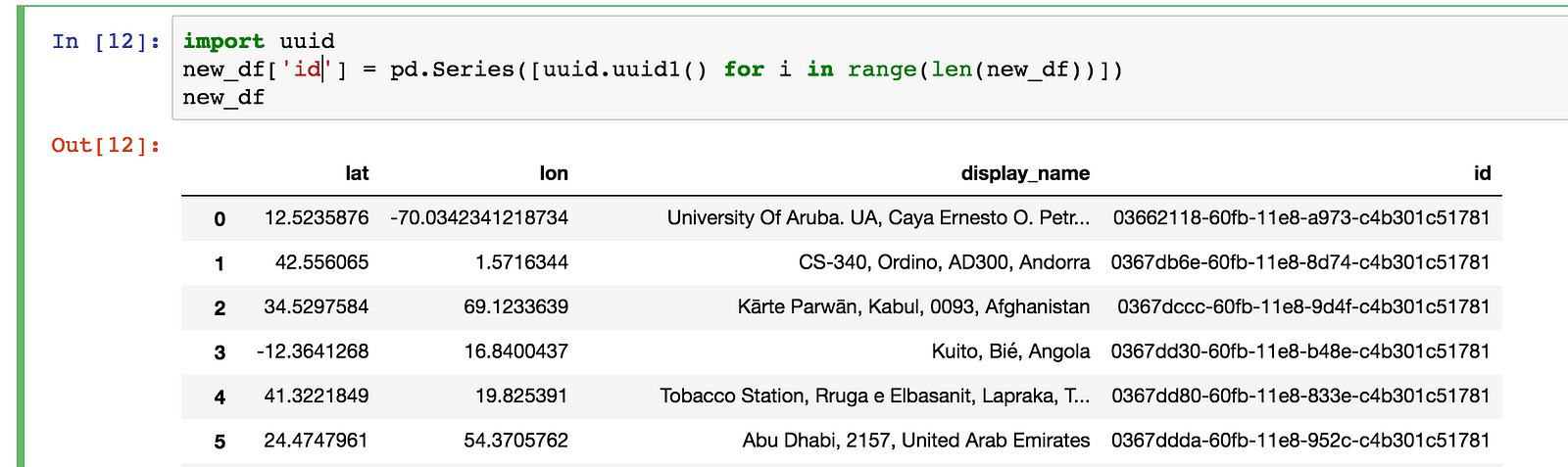
Let’s also add a Unique Identifier for each row

import uuidnew_df['id'] = pd.Series([uuid.uuid1() for i in range(len(new_df))])new_df

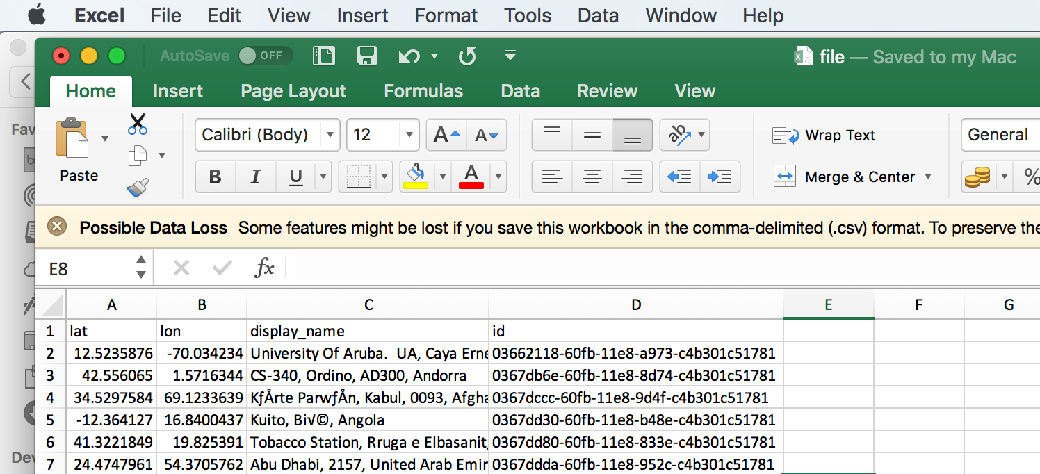
Step 6 — Generate CSV file and Upload to S3 Bucket

The following code creates a CSV file from Pandas DataFrame into the specified directory.

new_df.to_csv(path_or_buf=file_name,index=False)

The ‘to_csv’ method from Pandas automatically creates an Index column so we can avoid that by setting ‘index=False’.The CSV is now created and we can upload it to S3.

In this tutorial we will use TinyS3 <https://github.com/smore-inc/tinys3> which is a very easy to use library for working with S3. You can also use Boto3 if you wish.

import tinys3import osaccess_key = 'xxxxxxxxx'secret_key = 'xxxxxxxxx'endpoint = 'xxxxxxxx'Bucket_name = 'xxxxxxxx'

conn = tinys3.Connection(access_key, secret_key, tls=False, endpoint)

f = open(file_name,'rb')

conn.upload(file_name, f, Bucket_name)

f.close()os.remove(file_name)

The documentation is very self explanatory and basically says to add your AWS access key, secret access key and bucket name. You can then create a connection to S3 and upload the relevant file. We then delete the file from the drive by using ‘os.remove(file_name)’.

Step 7— Create Redshift Table and Copy Data into it

You will need to create a Redshift table before you can copy data into it. This can be done with standard SQL commands for PostgreSQL databases executed using Psycopg2 which is a PostgreSQL library for Python.

Create Table

import psycopg2    

my_db = 'xxxxxxx'my_host = 'xxxxxxx'my_port = 'xxxx'my_user = 'xxxxxxxx'my_password = 'xxxxxxx'

con = psycopg2.connect(dbname=my_db,host=my_host,port=my_port,user=my_user,password=my_password) 

cur = con.cursor()  

sql_query = "CREATE TABLE reverse_geocode_location (lat varchar(255),lon varchar(255),display_name varchar(255),id varchar(255),PRIMARY KEY (id));"

cur.execute(sql_query)con.commit()

cur.close()con.close()

Using Psycopg2 its very easy to execute SQL commands in Redshift or any other PostgreSQL engine database via Python. We first need to create a connection, then a cursor and lastly execute our SQL query. Don’t forget to close the connection to the database after the SQL query has been successfully executed.

Copy Data From S3 to Redshift

We are now ready for the last and final step in our Tutorial — Copy CSV file from S3 to Redshift. The reason we use COPY instead of using SQL Alchemy or other SQL clients because Redshift is optimised for columnar storage and this method is really fast to load data into it instead of loading the data row by row. We can use Psycopg2 once again for this.

Its very important to note that the column datatypes between the CSV file and Redshift table has to be the same and in the same order or the COPY command will fail. You can check any LOAD errors by reading from the STL_LOAD_ERRORS table.

import psycopg2

my_db = 'xxxxxxx'my_host = 'xxxxxxx'my_port = 'xxxx'my_user = 'xxxxxxxx'my_password = 'xxxxxxx'

con = psycopg2.connect(dbname=my_db,host=my_host,port=my_port,user=my_user,password=my_password)

cur = con.cursor()

sql_query = ""copy reverse_geocode_location from 's3://YOUR_BUCKET_NAME/YOUR_FILE_NAME' credentials 'aws_access_key_id=YOUR_ACCESS_KEY;aws_secret_access_key=YOUR_SECRET_ACCESS_KEY' csv IGNOREHEADER 1 NULL 'NaN' ACCEPTINVCHARS;""

cur.execute(sql_query)con.commit()

cur.close()con.close()

In the COPY command above we need to specify the bucket name, file name, security keys and a few flags. An explanation of the flags used can be found here:

Please Note: You need to grant correct IAM Role permissions in order to copy data from S3 into Redshift.

Step 8— Read data from your table to verify

Once you have successfully followed the above steps, you should now have the data copied into your Redshift table. You can verify it by reading the data using Psycopg2 in Python or any other SQL client.

select * from reverse_geocode_location

Conclusion and Next Steps

This tutorial covers some basics about using a Pandas Series as input to call a REST API and store the result in AWS Redshift. However if the data is scaled considerably its important to:

1. Subscribe to high performance, high volume handling API.
2. Reduce the in memory processing by writing to disk repeatedly or carry out parallel processing using libraries like Dask.
3. Use Apache Spark or other similar technologies to handle very large data processing.
4. Choose the database technology correctly based on performance requirement.

I hope this tutorial has been somewhat helpful, if you have any questions please get in touch via the comments.