數字訊號處理——MATLAB實驗(二)
阿新 • • 發佈:2018-12-20
實驗名稱:離散時間訊號和線性時不變離散時間系統的頻域分析
一、實驗目的:
熟悉Mat lab中的訊號處理工具箱及相關命令,掌握用Mat lab驗證離散時間傅立葉變換相關性質的方法;掌握用Mat lab分析離散時間系統頻域特性的方法並能繪製幅頻特性和相頻特性圖。
二、實驗內容及要求:
1. 離散時間訊號的頻域分析:
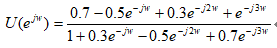
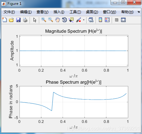
(1)修改程式P3.1,在範圍 內計算如下序列的離散時間傅立葉變換並繪製幅頻特性和相頻特性圖。
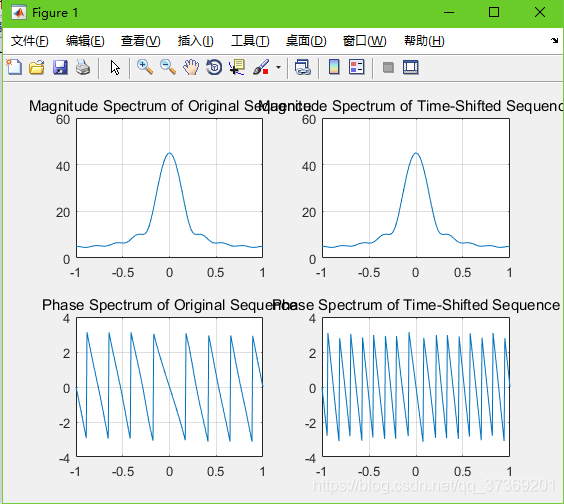
 (2)修改程式P3.2,D=8,驗證離散時間傅立葉變換的時移特性並繪圖。
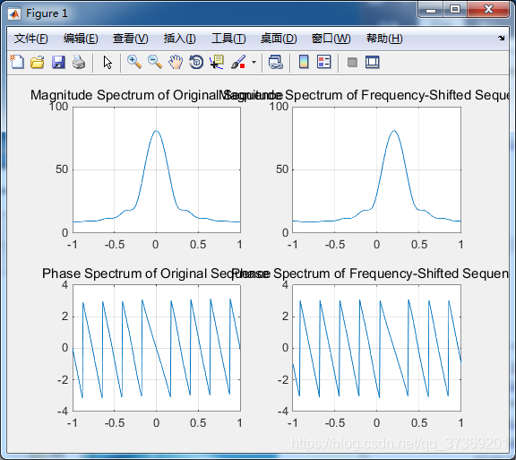
(3)修改程式P3.3,w = 0.2π ,驗證離散時間傅立葉變換的頻移特性並繪圖。
(2)修改程式P3.2,D=8,驗證離散時間傅立葉變換的時移特性並繪圖。
(3)修改程式P3.3,w = 0.2π ,驗證離散時間傅立葉變換的頻移特性並繪圖。
2. 線性時不變離散時間系統的頻域分析:
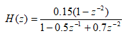
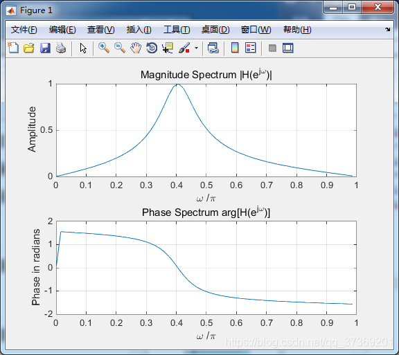
(1)修改程式P3.1,計算並畫出如下傳輸函式的頻率響應,它是哪種型別的濾波器?
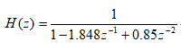
 (2)用Matlab畫出如下濾波器的零極點圖並分析穩定性。
三、實驗結果及問題回答:
1. 離散時間訊號的頻域分析:
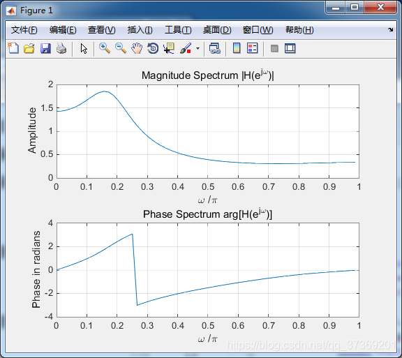
(1)實驗結果:
% Program P3_1
% Evaluation of the DTFT
clf;
% Compute the frequency samples of the DTFT
w = 0*pi:8*pi/511:pi;
num = [0.7 -0.5 0.3 1];den = [1 0.3 -0.5 0.7];
h = freqz(num, den, w);
% Plot the DTFT
subplot(2,1,1)
plot(w/pi,real(h));grid
title('Real part of H(e^{j\omega})')
xlabel('\omega /\pi');
ylabel('Amplitude');
subplot(2,1,2)
plot(w/pi,imag(h));grid
title('Imaginary part of H(e^{j\omega})')
xlabel('\omega /\pi');
ylabel('Amplitude');
pause
subplot(2,1,1)
plot(w/pi,abs(h));grid
title('Magnitude Spectrum |H(e^{j\omega})|')
xlabel('\omega /\pi');
ylabel('Amplitude');
subplot(2,1,2)
plot(w/pi,angle(h));grid
title('Phase Spectrum arg[H(e^{j\omega})]')
xlabel('\omega /\pi');
ylabel('Phase in radians');
 (2)實驗結果:
% Program P3_2
% Time-Shifting Properties of DTFT
clf;
w = -pi:2*pi/255:pi; wo = 0.4*pi; D = 8;
num = [1 2 3 4 5 6 7 8 9];
h1 = freqz(num, 1, w);
h2 = freqz([zeros(1,D) num], 1, w);
subplot(2,2,1)
plot(w/pi,abs(h1));grid
title('Magnitude Spectrum of Original Sequence')
subplot(2,2,2)
plot(w/pi,abs(h2));grid
title('Magnitude Spectrum of Time-Shifted Sequence')
subplot(2,2,3)
plot(w/pi,angle(h1));grid
title('Phase Spectrum of Original Sequence')
subplot(2,2,4)
plot(w/pi,angle(h2));grid
title('Phase Spectrum of Time-Shifted Sequence')
 (3)實驗結果:
% Program P3_3
% Frequency-Shifting Properties of DTFT
clf;
w = -pi:2*pi/255:pi; wo = 0.2*pi;
num1 = [1 3 5 7 9 11 13 15 17];
L = length(num1);
h1 = freqz(num1, 1, w);
n = 0:L-1;
num2 = exp(wo*i*n).*num1;
h2 = freqz(num2, 1, w);
subplot(2,2,1)
plot(w/pi,abs(h1));grid
title('Magnitude Spectrum of Original Sequence')
subplot(2,2,2)
plot(w/pi,abs(h2));grid
title('Magnitude Spectrum of Frequency-Shifted Sequence')
subplot(2,2,3)
plot(w/pi,angle(h1));grid
title('Phase Spectrum of Original Sequence')
subplot(2,2,4)
plot(w/pi,angle(h2));grid
title('Phase Spectrum of Frequency-Shifted Sequence')
2. 線性時不變離散時間系統的頻域分析:
(1)實驗結果:
% Program P3_1
% Evaluation of the DTFT
clf;
% Compute the frequency samples of the DTFT
w = 0*pi:8*pi/511:1*pi;
num = [0.15 0 -0.15];den = [1 -0.5 0.7];
h = freqz(num, den, w);
% Plot the DTFT
subplot(2,1,1)
plot(w/pi,real(h));grid
title('Real part of H(e^{j\omega})')
xlabel('\omega /\pi');
ylabel('Amplitude');
subplot(2,1,2)
plot(w/pi,imag(h));grid
title('Imaginary part of H(e^{j\omega})')
xlabel('\omega /\pi');
ylabel('Amplitude');
pause
subplot(2,1,1)
plot(w/pi,abs(h));grid
title('Magnitude Spectrum |H(e^{j\omega})|')
xlabel('\omega /\pi');
ylabel('Amplitude');
subplot(2,1,2)
plot(w/pi,angle(h));grid
title('Phase Spectrum arg[H(e^{j\omega})]')
xlabel('\omega /\pi');
ylabel('Phase in radians');
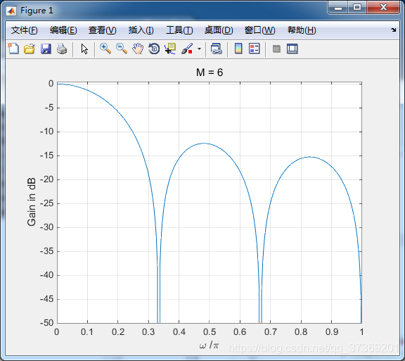
 (2)實驗結果:
% Program P4_2
% Gain Response of a Moving Average Lowpass Filter
clf;
M = 6;
num = ones(1,M)/M;
[g,w] = gain(num,1);
plot(w/pi,g);grid
axis([0 1 -50 0.5])
xlabel('\omega /\pi');ylabel('Gain in dB');
title(['M = ', num2str(M)])

function [g,w] = gain(num,den)
% Computes the gain function in dB of a
% transfer function at 256 equally spaced points
% on the top half of the unit circle
% Numerator coefficients are in vector num
% Denominator coefficients are in vector den
% Frequency values are returned in vector w
% Gain values are returned in vector g
w = 0:pi/255:pi;
h = freqz(num,den,w);
g = 20*log10(abs(h));
 (3)實驗結果:
% Program P3_1
% Evaluation of the DTFT
clf;
% Compute the frequency samples of the DTFT
w = 0*pi:8*pi/511:1*pi;
num = [1 0 0];den = [1 -1.848 0.85 0.7];
h = freqz(num, den, w);
% Plot the DTFT
subplot(2,1,1)
plot(w/pi,real(h));grid
title('Real part of H(e^{j\omega})')
xlabel('\omega /\pi');
ylabel('Amplitude');
subplot(2,1,2)
plot(w/pi,imag(h));grid
title('Imaginary part of H(e^{j\omega})')
xlabel('\omega /\pi');
ylabel('Amplitude');
pause
subplot(2,1,1)
plot(w/pi,abs(h));grid
title('Magnitude Spectrum |H(e^{j\omega})|')
xlabel('\omega /\pi');
ylabel('Amplitude');
subplot(2,1,2)
plot(w/pi,angle(h));grid
title('Phase Spectrum arg[H(e^{j\omega})]')
xlabel('\omega /\pi');
ylabel('Phase in radians');