CS231N softmax
作業講解
求損失Loss
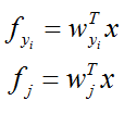
線性模型:y=Wxy=Wx
  scores = X.dot(W)
  correct_class_score = scores[np.arange(num_train),y].reshape(num_train,1)
  exp_sum = np.sum(np.exp(scores),axis=1).reshape(num_train,1)
  loss += np.sum(np.log(exp_sum) - correct_class_score)
  loss /= num_train
loss += 0.5 * reg * np.sum(W * W)- 1
- 2
- 3
- 4
- 5
- 6
求梯度dW
Loss:Li=−wixi+log∑jewjxjLi=−wixi+log∑jewjxj
對W求導:
  margin = np.exp(scores) / exp_sum
  margin[np.arange(num_train),y] += -1
  dW = X.T.dot(margin)
  dW /= num_train
dW += reg * W- 1
- 2
- 3
- 4
- 5
求導具體過程
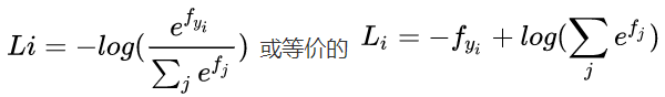
梯度【參考這裡】: Softmax與SVM,只是換了個損失函式,求導的思想類同,也需要分兩種情況 j==yiyi , Softmax損失函式和求導步驟公式如下: 具體看一下這個損失函式,這裡的 f 對應著scores:
所以,這裡要運用鏈式法則,對梯度求偏導一共有兩層:
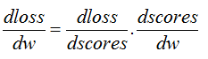
dscoresdwdscoresdw:
j!=yiyi 針對錯誤項分母進行求偏導:
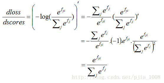
j==yiyi 針對分子進行求偏導:
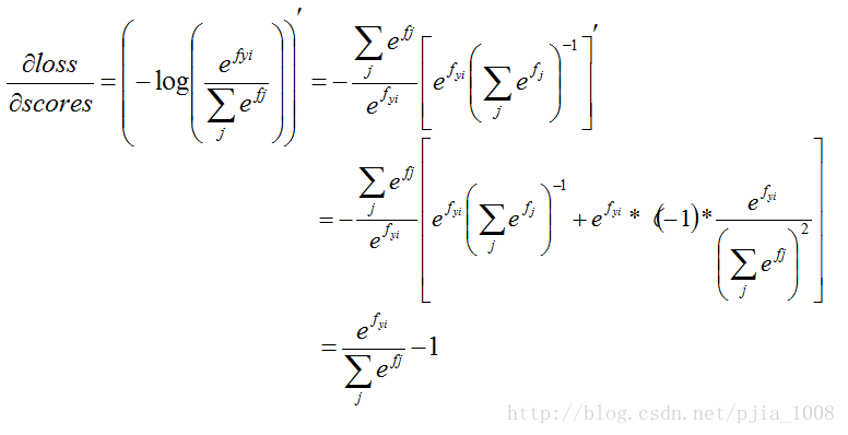
dlossdscoresdlossdscores就完成了softmax的梯度求導了!
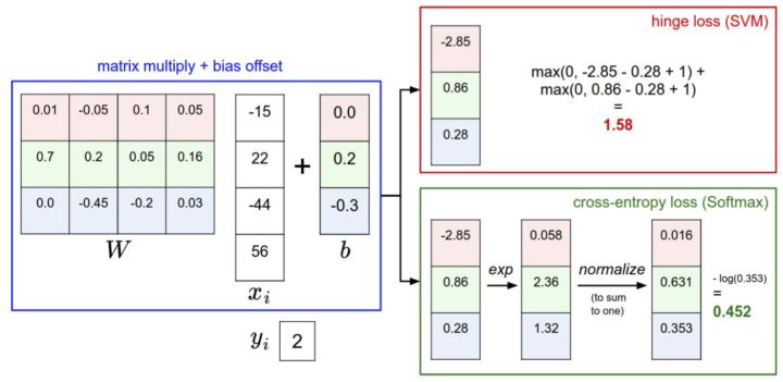
SVM與Softmax分類器的比較
對於學習過二元邏輯迴歸分類器的讀者來說,Softmax分類器就可以理解為邏輯迴歸分類器面對多個分類的一般化歸納。SVM將輸出 f
在上式中,使用 fjfj。
下圖有助於區分這 Softmax和SVM這兩種分類器:
總體程式碼展示
開啟softmax.ipynb:
import random
import numpy as np
from cs231n.data_utils import load_CIFAR10
import matplotlib.pyplot as plt
%matplotlib inline
plt.rcParams['figure.figsize'] = (10.0, 8.0) # set default size of plots
plt.rcParams['image.interpolation'] = 'nearest'
plt.rcParams['image.cmap'] = 'gray'- 1
- 2
- 3
- 4
- 5
- 6
- 7
- 8
載入資料並預處理
def get_CIFAR10_data(num_training=49000, num_validation=1000, num_test=1000, num_dev=500):
  """
  Load the CIFAR-10 dataset from disk and perform preprocessing to prepare
  it for the linear classifier. These are the same steps as we used for the
  SVM, but condensed to a single function.
  """
  # Load the raw CIFAR-10 data
  cifar10_dir = 'cs231n/datasets/cifar-10-batches-py'
  X_train, y_train, X_test, y_test = load_CIFAR10(cifar10_dir)

  # subsample the data
  mask = range(num_training, num_training + num_validation)
  X_val = X_train[mask]
  y_val = y_train[mask]
  mask = range(num_training)
  X_train = X_train[mask]
  y_train = y_train[mask]
  mask = range(num_test)
  X_test = X_test[mask]
  y_test = y_test[mask]
  mask = np.random.choice(num_training, num_dev, replace=False)
  X_dev = X_train[mask]
  y_dev = y_train[mask]

  # Preprocessing: reshape the image data into rows
  X_train = np.reshape(X_train, (X_train.shape[0], -1))
  X_val = np.reshape(X_val, (X_val.shape[0], -1))
  X_test = np.reshape(X_test, (X_test.shape[0], -1))
  X_dev = np.reshape(X_dev, (X_dev.shape[0], -1))

  # Normalize the data: subtract the mean image
  mean_image = np.mean(X_train, axis = 0)
  X_train -= mean_image
  X_val -= mean_image
  X_test -= mean_image
  X_dev -= mean_image

  # add bias dimension and transform into columns
  X_train = np.hstack([X_train, np.ones((X_train.shape[0], 1))])
  X_val = np.hstack([X_val, np.ones((X_val.shape[0], 1))])
  X_test = np.hstack([X_test, np.ones((X_test.shape[0], 1))])
  X_dev = np.hstack([X_dev, np.ones((X_dev.shape[0], 1))])

  return X_train, y_train, X_val, y_val, X_test, y_test, X_dev, y_dev


# Invoke the above function to get our data.
X_train, y_train, X_val, y_val, X_test, y_test, X_dev, y_dev = get_CIFAR10_data()
print ('Train data shape: ', X_train.shape)
print ('Train labels shape: ', y_train.shape)
print ('Validation data shape: ', X_val.shape)
print ('Validation labels shape: ', y_val.shape)
print ('Test data shape: ', X_test.shape)
print ('Test labels shape: ', y_test.shape)
print ('dev data shape: ', X_dev.shape)
print ('dev labels shape: ', y_dev.shape)- 1
- 2
- 3
- 4
- 5
- 6
- 7
- 8
- 9
- 10
- 11
- 12
- 13
- 14
- 15
- 16
- 17
- 18
- 19
- 20
- 21
- 22
- 23
- 24
- 25
- 26
- 27
- 28
- 29
- 30
- 31
- 32
- 33
- 34
- 35
- 36
- 37
- 38
- 39
- 40
- 41
- 42
- 43
- 44
- 45
- 46
- 47
- 48
- 49
- 50
- 51
- 52
- 53
- 54
- 55
- 56
OUTPUT: Train data shape: (49000, 3073) Train labels shape: (49000,) Validation data shape: (1000, 3073) Validation labels shape: (1000,) Test data shape: (1000, 3073) Test labels shape: (1000,) dev data shape: (500, 3073) dev labels shape: (500,)
Softmax分類器的實現
開啟cs231n\classifiers資料夾中的 softmax.py 完成SVM的實現程式碼。
方法一:
import numpy as np

def softmax_loss_naive(W, X, y, reg):

  # Initialize the loss and gradient to zero.
  loss = 0.0
  dW = np.zeros_like(W)

  num_classes = W.shape[1]
  num_train = X.shape[0]
  for i in range(num_train):
      scores = X[i].dot(W)
      correct_class = y[i]
      exp_scores = np.zeros_like(scores)
      row_sum = 0
      for j in range(num_classes):
          exp_scores[j] = np.exp(scores[j])
          row_sum += exp_scores[j]
      loss += -np.log(exp_scores[correct_class]/row_sum)
      #compute dW loops:
      for k in range(num_classes):
        if k != correct_class:
          dW[:,k] += exp_scores[k] / row_sum * X[i]
        else:
          dW[:,k] += (exp_scores[correct_class]/row_sum - 1) * X[i]
  loss /= num_train
  reg_loss = 0.5 * reg * np.sum(W**2)
  loss += reg_loss
  dW /= num_train
  dW += reg * W

return loss, dW- 1
- 2
- 3
- 4
- 5
- 6
- 7
- 8
- 9
- 10
- 11
- 12
- 13
- 14
- 15
- 16
- 17
- 18
- 19
- 20
- 21
- 22
- 23
- 24
- 25
- 26
- 27
- 28
- 29
- 30
- 31
- 32
方法二 向量化:
def softmax_loss_vectorized(W, X, y, reg):

  # Initialize the loss and gradient to zero.
  loss = 0.0
  dW = np.zeros_like(W)

  num_train = X.shape[0]
  scores = X.dot(W)
  correct_class_score = scores[np.arange(num_train),y].reshape(num_train,1)
  exp_sum = np.sum(np.exp(scores),axis=1).reshape(num_train,1)
  loss += np.sum(np.log(exp_sum) - correct_class_score)
  loss /= num_train
  loss += 0.5 * reg * np.sum(W * W)

  #compute gradient
  margin = np.exp(scores) / exp_sum
  margin[np.arange(num_train),y] += -1
  dW = X.T.dot(margin)
  dW /= num_train
  dW += reg * W

return loss, dW- 1
- 2
- 3
- 4
- 5
- 6
- 7
- 8
- 9
- 10
- 11
- 12
- 13
- 14
- 15
- 16
- 17
- 18
- 19
- 20
- 21
- 22
梯度檢查
返回softmax.ipynb
# Complete the implementation of softmax_loss_naive and implement a (naive)
# version of the gradient that uses nested loops.
loss, grad = softmax_loss_naive(W, X_dev, y_dev, 0.0)

# As we did for the SVM, use numeric gradient checking as a debugging tool.
# The numeric gradient should be close to the analytic gradient.
from cs231n.gradient_check import grad_check_sparse
f = lambda w: softmax_loss_naive(w, X_dev, y_dev, 0.0)[0]
grad_numerical = grad_check_sparse(f, W, grad, 10)

# similar to SVM case, do another gradient check with regularization
loss, grad = softmax_loss_naive(W, X_dev, y_dev, 1e2)
f = lambda w: softmax_loss_naive(w, X_dev, y_dev, 1e2)[0]
grad_numerical = grad_check_sparse(f, W, grad, 10)- 1
- 2
- 3
- 4
- 5
- 6
- 7
- 8
- 9
- 10
- 11
- 12
- 13
- 14
其中,梯度檢查函式為:
def grad_check_sparse(f, x, analytic_grad, num_checks=10, h=1e-5):
  """
  sample a few random elements and only return numerical
  in this dimensions.
  """

  for i in range(num_checks):
    ix = tuple([randrange(m) for m in x.shape])

    oldval = x[ix]
    x[ix] = oldval + h # increment by h
    fxph = f(x) # evaluate f(x + h)
    x[ix] = oldval - h # increment by h
    fxmh = f(x) # evaluate f(x - h)
    x[ix] = oldval # reset

    grad_numerical = (fxph - fxmh) / (2 * h)
    grad_analytic = analytic_grad[ix]
    rel_error = abs(grad_numerical - grad_analytic) / (abs(grad_numerical) + abs(grad_analytic))
print ('numerical: %f analytic: %f, relative error: %e' % (grad_numerical, grad_analytic, rel_error))- 1
- 2
- 3
- 4
- 5
- 6
- 7
- 8
- 9
- 10
- 11
- 12
- 13
- 14
- 15
- 16
- 17
- 18
- 19
- 20
計算loss和梯度
tic = time.time()
loss_naive, grad_naive = softmax_loss_naive(W, X_dev, y_dev, 0.00001)
toc = time.time()
print ('naive loss: %e computed in %fs' % (loss_naive, toc - tic))

from cs231n.classifiers.softmax import softmax_loss_vectorized
tic = time.time()
loss_vectorized, grad_vectorized = softmax_loss_vectorized(W, X_dev, y_dev, 0.00001)
toc = time.time()
print ('vectorized loss: %e computed in %fs' % (loss_vectorized, toc - tic))

# As we did for the SVM, we use the Frobenius norm to compare the two versions
# of the gradient.
grad_difference = np.linalg.norm(grad_naive - grad_vectorized, ord='fro')
print ('Loss difference: %f' % np.abs(loss_naive - loss_vectorized))
print ('Gradient difference: %f' % grad_difference)- 1
- 2
- 3
- 4
- 5
- 6
- 7
- 8
- 9
- 10
- 11
- 12
- 13
- 14
- 15
- 16
OUTPUT: naive loss: 2.371882e+00 computed in 0.189139s vectorized loss: 2.371882e+00 computed in 0.026646s Loss difference: 0.000000 Gradient difference: 0.000000
隨機梯度下降
與SVM一樣,在linear_classifier.py 檔案中實現SGD函式
預測準確度
與SVM一樣,在linear_classifier.py 檔案中實現【predict】函式
利用交叉驗證集調整超引數
from cs231n.classifiers import Softmax
results = {}
best_val = -1
best_softmax = None
learning_rates = [1e-7, 5e-7]
regularization_strengths = [5e4, 1e8]

################################################################################
# TODO:                                                                        #
# Use the validation set to set the learning rate and regularization strength. #
# This should be identical to the validation that you did for the SVM; save    #
# the best trained softmax classifer in best_softmax.                          #
################################################################################
iters = 2000
for lr in learning_rates:
    for rs in regularization_strengths:
        softmax = Softmax()
        softmax.train(X_train, y_train, learning_rate=lr, reg=rs, num_iters=iters)

        y_train_pred = softmax.predict(X_train)
        acc_train = np.mean(y_train == y_train_pred)
        y_val_pred = softmax.predict(X_val)
        acc_val = np.mean(y_val == y_val_pred)

        results[(lr, rs)] = (acc_train, acc_val)

        if best_val < acc_val:
            best_val = acc_val
            best_softmax = softmax
################################################################################
#                              END OF YOUR CODE                                #
################################################################################

# Print out results.
for lr, reg in sorted(results):
    train_accuracy, val_accuracy = results[(lr, reg)]
    print ('lr %e reg %e train accuracy: %f val accuracy: %f' % (
                lr, reg, train_accuracy, val_accuracy))

print ('best validation accuracy achieved during cross-validation: %f' % best_val)- 1
- 2
- 3
- 4
- 5
- 6
- 7
- 8
- 9
- 10
- 11
- 12
- 13
- 14
- 15
- 16
- 17
- 18
- 19
- 20
- 21
- 22
- 23
- 24
- 25
- 26
- 27
- 28
- 29
- 30
- 31
- 32
- 33
- 34
- 35
- 36
- 37
- 38
- 39
- 40
OUTPUT: lr 1.000000e-07 reg 5.000000e+04 train accuracy: 0.326796 val accuracy: 0.343000 lr 1.000000e-07 reg 1.000000e+08 train accuracy: 0.100265 val accuracy: 0.087000 lr 5.000000e-07 reg 5.000000e+04 train accuracy: 0.331020 val accuracy: 0.355000 lr 5.000000e-07 reg 1.000000e+08 train accuracy: 0.100265 val accuracy: 0.087000 best validation accuracy achieved during cross-validation: 0.355000
在測試集上驗證
# evaluate on test set
# Evaluate the best softmax on test set
y_test_pred = best_softmax.predict(X_test)
test_accuracy = np.mean(y_test == y_test_pred)
print ('softmax on raw pixels final test set accuracy: %f' % (test_accuracy, ))- 1
- 2
- 3
- 4
- 5
OUTPUT: softmax on raw pixels final test set accuracy: 0.339000
# Visualize the learned weights for each class
w = best_softmax.W[:-1,:] # strip out the bias
w = w.reshape(32, 32, 3, 10)

w_min, w_max = np.min(w), np.max(w)

classes = ['plane', 'car', 'bird', 'cat', 'deer', 'dog', 'frog', 'horse', 'ship', 'truck']
for i in range(10):
  plt.subplot(2, 5, i + 1)

  # Rescale the weights to be between 0 and 255
  wimg = 255.0 * (w[:, :, :, i].squeeze() - w_min) / (w_max - w_min)
  plt.imshow(wimg.astype('uint8'))
  plt.axis('off')
plt.title(classes[i])- 1
- 2
- 3
- 4
- 5
- 6
- 7
- 8
- 9
- 10
- 11
- 12
- 13
- 14
- 15
OUTPUT: