摘要： 本文主要和大家分享如何使用Tensorflow從頭開始構建和訓練卷積神經網路。這樣就可以將這個知識作為一個構建塊來創造有趣的深度學習應用程式了。

0. 簡介

在過去，我寫的主要都是“傳統類”的機器學習文章，如樸素貝葉斯分類、邏輯迴歸和Perceptron演算法。在過去的一年中，我一直在研究深度學習技術，因此，我想和大家分享一下如何使用Tensorflow從頭開始構建和訓練卷積神經網路。這樣，我們以後就可以將這個知識作為一個構建塊來創造有趣的深度學習應用程式了。

為此，你需要安裝Tensorflow（請參閱安裝說明），你還應該對Python程式設計和卷積神經網路背後的理論有一個基本的瞭解。安裝完Tensorflow之後，你可以在不依賴GPU的情況下執行一個較小的神經網路，但對於更深層次的神經網路，就需要用到GPU的計算能力了。

在網際網路上有很多解釋卷積神經網路工作原理方面的網站和課程，其中有一些還是很不錯的，圖文並茂、易於理解[點選此處獲取更多資訊]。我在這裡就不再解釋相同的東西，所以在開始閱讀下文之前，請提前瞭解卷積神經網路的工作原理。例如：

• 什麼是卷積層，卷積層的過濾器是什麼？
• 什麼是啟用層（ReLu層（應用最廣泛的）、S型啟用或tanh）？
• 什麼是池層（最大池/平均池），什麼是dropout？
• 隨機梯度下降的工作原理是什麼？

本文內容如下：

1. Tensorflow基礎

   • 1.1 常數和變數
   • 1.2 Tensorflow中的圖和會話
   • 1.3 佔位符和feed_dicts

2. Tensorflow中的神經網路

   • 2.1 介紹
   • 2.2 資料載入
   • 2.3 建立一個簡單的一層神經網路
   • 2.4 Tensorflow的多個方面
   • 2.5 建立LeNet5卷積神經網路
   • 2.6 影響層輸出大小的引數
   • 2.7 調整LeNet5架構
   • 2.8 學習速率和優化器的影響

3. Tensorflow中的深度神經網路

   • 3.1 AlexNet
   • 3.2 VGG Net-16
   • 3.3 AlexNet效能
4. 結語

1. Tensorflow 基礎

在這裡，我將向以前從未使用過Tensorflow的人做一個簡單的介紹。如果你想要立即開始構建神經網路，或者已經熟悉Tensorflow，可以直接跳到第2節。如果你想了解更多有關Tensorflow的資訊，你還可以檢視這個程式碼庫，或者閱讀斯坦福大學CS20SI課程的講義1和講義2。

1.1 常量與變數

Tensorflow中最基本的單元是常量、變數和佔位符。

tf.constant()和tf.Variable()之間的區別很清楚；一個常量有著恆定不變的值，一旦設定了它，它的值不能被改變。而變數的值可以在設定完成後改變，但變數的資料型別和形狀無法改變。

#We can create constants and variables of different types. 
#However, the different types do not mix well together.
a = tf.constant(2, tf.int16)
b = tf.constant(4, tf.float32)
c = tf.constant(8, tf.float32)

d = tf.Variable(2, tf.int16)
e = tf.Variable(4, tf.float32)
f = tf.Variable(8, tf.float32)

#we can perform computations on variable of the same type: e + f
#but the following can not be done: d + e

#everything in Tensorflow is a tensor, these can have different dimensions:
#0D, 1D, 2D, 3D, 4D, or nD-tensors
g = tf.constant(np.zeros(shape=(2,2), dtype=np.float32)) #does work

h = tf.zeros([11], tf.int16)
i = tf.ones([2,2], tf.float32)
j = tf.zeros([1000,4,3], tf.float64)

k = tf.Variable(tf.zeros([2,2], tf.float32))
l = tf.Variable(tf.zeros([5,6,5], tf.float32))

除了tf.zeros()和tf.ones()能夠建立一個初始值為0或1的張量（見這裡）之外，還有一個tf.random_normal()函式，它能夠建立一個包含多個隨機值的張量，這些隨機值是從正態分佈中隨機抽取的（預設的分佈均值為0.0，標準差為1.0）。

另外還有一個tf.truncated_normal()函式，它建立了一個包含從截斷的正態分佈中隨機抽取的值的張量，其中下上限是標準偏差的兩倍。

有了這些知識，我們就可以建立用於神經網路的權重矩陣和偏差向量了。

weights = tf.Variable(tf.truncated_normal([256 * 256, 10]))
biases = tf.Variable(tf.zeros([10]))
print(weights.get_shape().as_list())
print(biases.get_shape().as_list())
>>>[65536, 10]
>>>[10]

1.2 Tensorflow 中的圖與會話

在Tensorflow中，所有不同的變數以及對這些變數的操作都儲存在圖（Graph）中。在構建了一個包含針對模型的所有計算步驟的圖之後，就可以在會話（Session）中執行這個圖了。會話可以跨CPU和GPU分配所有的計算。

graph = tf.Graph()
with graph.as_default():
    a = tf.Variable(8, tf.float32)
    b = tf.Variable(tf.zeros([2,2], tf.float32))
    
with tf.Session(graph=graph) as session:
    tf.global_variables_initializer().run()
    print(f)
    print(session.run(f))
    print(session.run(k))

>>> <tf.Variable 'Variable_2:0' shape=() dtype=int32_ref>
>>> 8
>>> [[ 0.  0.]
>>>  [ 0.  0.]]

1.3 佔位符 與 feed_dicts

我們已經看到了用於建立常量和變數的各種形式。Tensorflow中也有佔位符，它不需要初始值，僅用於分配必要的記憶體空間。 在一個會話中，這些佔位符可以通過feed_dict填入（外部）資料。

以下是佔位符的使用示例。

list_of_points1_ = [[1,2], [3,4], [5,6], [7,8]]
list_of_points2_ = [[15,16], [13,14], [11,12], [9,10]]
list_of_points1 = np.array([np.array(elem).reshape(1,2) for elem in list_of_points1_])
list_of_points2 = np.array([np.array(elem).reshape(1,2) for elem in list_of_points2_])

graph = tf.Graph()
with graph.as_default():   
    #we should use a tf.placeholder() to create a variable whose value you will fill in later (during session.run()). 
    #this can be done by 'feeding' the data into the placeholder.
    #below we see an example of a method which uses two placeholder arrays of size [2,1] to calculate the eucledian distance

    point1 = tf.placeholder(tf.float32, shape=(1, 2))
    point2 = tf.placeholder(tf.float32, shape=(1, 2))
    
    def calculate_eucledian_distance(point1, point2):
        difference = tf.subtract(point1, point2)
        power2 = tf.pow(difference, tf.constant(2.0, shape=(1,2)))
        add = tf.reduce_sum(power2)
        eucledian_distance = tf.sqrt(add)
        return eucledian_distance
    
    dist = calculate_eucledian_distance(point1, point2)
    
with tf.Session(graph=graph) as session:
    tf.global_variables_initializer().run()   
    for ii in range(len(list_of_points1)):
        point1_ = list_of_points1[ii]
        point2_ = list_of_points2[ii]
        feed_dict = {point1 : point1_, point2 : point2_}
        distance = session.run([dist], feed_dict=feed_dict)
        print("the distance between {} and {} -> {}".format(point1_, point2_, distance))

>>> the distance between [[1 2]] and [[15 16]] -> [19.79899]
>>> the distance between [[3 4]] and [[13 14]] -> [14.142136]
>>> the distance between [[5 6]] and [[11 12]] -> [8.485281]
>>> the distance between [[7 8]] and [[ 9 10]] -> [2.8284271]

2. Tensorflow 中的神經網路

2.1 簡介

包含神經網路的圖（如上圖所示）應包含以下步驟：

1. 輸入資料集：訓練資料集和標籤、測試資料集和標籤（以及驗證資料集和標籤）。
   測試和驗證資料集可以放在tf.constant()中。而訓練資料集被放在tf.placeholder()中，這樣它可以在訓練期間分批輸入（隨機梯度下降）。
2. 神經網路模型及其所有的層。這可以是一個簡單的完全連線的神經網路，僅由一層組成，或者由5、9、16層組成的更復雜的神經網路。
3. 權重矩陣和偏差向量以適當的形狀進行定義和初始化。（每層一個權重矩陣和偏差向量）
4. 損失值：模型可以輸出分對數向量（估計的訓練標籤），並通過將分對數與實際標籤進行比較，計算出損失值（具有交叉熵函式的softmax）。損失值表示估計訓練標籤與實際訓練標籤的接近程度，並用於更新權重值。
5. 優化器：它用於將計算得到的損失值來更新反向傳播演算法中的權重和偏差。

2.2 資料載入

下面我們來載入用於訓練和測試神經網路的資料集。為此，我們要下載MNIST和CIFAR-10資料集。 MNIST資料集包含了6萬個手寫數字影象，其中每個影象大小為28 x 28 x 1（灰度）。 CIFAR-10資料集也包含了6萬個影象（3個通道），大小為32 x 32 x 3，包含10個不同的物體（飛機、汽車、鳥、貓、鹿、狗、青蛙、馬、船、卡車）。 由於兩個資料集中都有10個不同的物件，所以這兩個資料集都包含10個標籤。

首先，我們來定義一些方便載入資料和格式化資料的方法。

def randomize(dataset, labels):
    permutation = np.random.permutation(labels.shape[0])
    shuffled_dataset = dataset[permutation, :, :]
    shuffled_labels = labels[permutation]
    return shuffled_dataset, shuffled_labels

def one_hot_encode(np_array):
    return (np.arange(10) == np_array[:,None]).astype(np.float32)

def reformat_data(dataset, labels, image_width, image_height, image_depth):
    np_dataset_ = np.array([np.array(image_data).reshape(image_width, image_height, image_depth) for image_data in dataset])
    np_labels_ = one_hot_encode(np.array(labels, dtype=np.float32))
    np_dataset, np_labels = randomize(np_dataset_, np_labels_)
    return np_dataset, np_labels

def flatten_tf_array(array):
    shape = array.get_shape().as_list()
    return tf.reshape(array, [shape[0], shape[1] * shape[2] * shape[3]])

def accuracy(predictions, labels):
    return (100.0 * np.sum(np.argmax(predictions, 1) == np.argmax(labels, 1)) / predictions.shape[0])

這些方法可用於對標籤進行獨熱碼編碼、將資料載入到隨機陣列中、扁平化矩陣（因為完全連線的網路需要一個扁平矩陣作為輸入）：

在我們定義了這些必要的函式之後，我們就可以這樣載入MNIST和CIFAR-10資料集了：

mnist_folder = './data/mnist/'
mnist_image_width = 28
mnist_image_height = 28
mnist_image_depth = 1
mnist_num_labels = 10

mndata = MNIST(mnist_folder)
mnist_train_dataset_, mnist_train_labels_ = mndata.load_training()
mnist_test_dataset_, mnist_test_labels_ = mndata.load_testing()

mnist_train_dataset, mnist_train_labels = reformat_data(mnist_train_dataset_, mnist_train_labels_, mnist_image_size, mnist_image_size, mnist_image_depth)
mnist_test_dataset, mnist_test_labels = reformat_data(mnist_test_dataset_, mnist_test_labels_, mnist_image_size, mnist_image_size, mnist_image_depth)

print("There are {} images, each of size {}".format(len(mnist_train_dataset), len(mnist_train_dataset[0])))
print("Meaning each image has the size of 28*28*1 = {}".format(mnist_image_size*mnist_image_size*1))
print("The training set contains the following {} labels: {}".format(len(np.unique(mnist_train_labels_)), np.unique(mnist_train_labels_)))

print('Training set shape', mnist_train_dataset.shape, mnist_train_labels.shape)
print('Test set shape', mnist_test_dataset.shape, mnist_test_labels.shape)

train_dataset_mnist, train_labels_mnist = mnist_train_dataset, mnist_train_labels
test_dataset_mnist, test_labels_mnist = mnist_test_dataset, mnist_test_labels

######################################################################################

cifar10_folder = './data/cifar10/'
train_datasets = ['data_batch_1', 'data_batch_2', 'data_batch_3', 'data_batch_4', 'data_batch_5', ]
test_dataset = ['test_batch']
c10_image_height = 32
c10_image_width = 32
c10_image_depth = 3
c10_num_labels = 10

with open(cifar10_folder + test_dataset[0], 'rb') as f0:
    c10_test_dict = pickle.load(f0, encoding='bytes')

c10_test_dataset, c10_test_labels = c10_test_dict[b'data'], c10_test_dict[b'labels']
test_dataset_cifar10, test_labels_cifar10 = reformat_data(c10_test_dataset, c10_test_labels, c10_image_size, c10_image_size, c10_image_depth)

c10_train_dataset, c10_train_labels = [], []
for train_dataset in train_datasets:
    with open(cifar10_folder + train_dataset, 'rb') as f0:
        c10_train_dict = pickle.load(f0, encoding='bytes')
        c10_train_dataset_, c10_train_labels_ = c10_train_dict[b'data'], c10_train_dict[b'labels']
 
        c10_train_dataset.append(c10_train_dataset_)
        c10_train_labels += c10_train_labels_

c10_train_dataset = np.concatenate(c10_train_dataset, axis=0)
train_dataset_cifar10, train_labels_cifar10 = reformat_data(c10_train_dataset, c10_train_labels, c10_image_size, c10_image_size, c10_image_depth)
del c10_train_dataset
del c10_train_labels

print("The training set contains the following labels: {}".format(np.unique(c10_train_dict[b'labels'])))
print('Training set shape', train_dataset_cifar10.shape, train_labels_cifar10.shape)
print('Test set shape', test_dataset_cifar10.shape, test_labels_cifar10.shape)

你可以從Yann LeCun的網站下載MNIST資料集。下載並解壓縮之後，可以使用python-mnist 工具來載入資料。 CIFAR-10資料集可以從這裡下載。

2.3 建立一個簡單的一層神經網路

神經網路最簡單的形式是一層線性全連線神經網路（FCNN， Fully Connected Neural Network）。 在數學上它由一個矩陣乘法組成。

最好是在Tensorflow中從這樣一個簡單的NN開始，然後再去研究更復雜的神經網路。 當我們研究那些更復雜的神經網路的時候，只是圖的模型（步驟2）和權重（步驟3）發生了改變，其他步驟仍然保持不變。

我們可以按照如下程式碼製作一層FCNN：

image_width = mnist_image_width
image_height = mnist_image_height
image_depth = mnist_image_depth
num_labels = mnist_num_labels 

#the dataset
train_dataset = mnist_train_dataset
train_labels = mnist_train_labels 
test_dataset = mnist_test_dataset
test_labels = mnist_test_labels 

#number of iterations and learning rate
num_steps = 10001
display_step = 1000
learning_rate = 0.5

graph = tf.Graph()
with graph.as_default():
    #1) First we put the input data in a Tensorflow friendly form. 
    tf_train_dataset = tf.placeholder(tf.float32, shape=(batch_size, image_width, image_height, image_depth))
    tf_train_labels = tf.placeholder(tf.float32, shape = (batch_size, num_labels))
    tf_test_dataset = tf.constant(test_dataset, tf.float32)
  
    #2) Then, the weight matrices and bias vectors are initialized
    #as a default, tf.truncated_normal() is used for the weight matrix and tf.zeros() is used for the bias vector.
    weights = tf.Variable(tf.truncated_normal([image_width * image_height * image_depth, num_labels]), tf.float32)
    bias = tf.Variable(tf.zeros([num_labels]), tf.float32)
  
    #3) define the model:
    #A one layered fccd simply consists of a matrix multiplication
    def model(data, weights, bias):
        return tf.matmul(flatten_tf_array(data), weights) + bias

    logits = model(tf_train_dataset, weights, bias)

    #4) calculate the loss, which will be used in the optimization of the weights
    loss = tf.reduce_mean(tf.nn.softmax_cross_entropy_with_logits(logits=logits, labels=tf_train_labels))

    #5) Choose an optimizer. Many are available.
    optimizer = tf.train.GradientDescentOptimizer(learning_rate).minimize(loss)

    #6) The predicted values for the images in the train dataset and test dataset are assigned to the variables train_prediction and test_prediction. 
    #It is only necessary if you want to know the accuracy by comparing it with the actual values. 
    train_prediction = tf.nn.softmax(logits)
    test_prediction = tf.nn.softmax(model(tf_test_dataset, weights, bias))


with tf.Session(graph=graph) as session:
    tf.global_variables_initializer().run()
    print('Initialized')
    for step in range(num_steps):
        _, l, predictions = session.run([optimizer, loss, train_prediction])
        if (step % display_step == 0):
            train_accuracy = accuracy(predictions, train_labels[:, :])
            test_accuracy = accuracy(test_prediction.eval(), test_labels)
            message = "step {:04d} : loss is {:06.2f}, accuracy on training set {:02.2f} %, accuracy on test set {:02.2f} %".format(step, l, train_accuracy, test_accuracy)
            print(message)

>>> Initialized
>>> step 0000 : loss is 2349.55, accuracy on training set 10.43 %, accuracy on test set 34.12 %
>>> step 0100 : loss is 3612.48, accuracy on training set 89.26 %, accuracy on test set 90.15 %
>>> step 0200 : loss is 2634.40, accuracy on training set 91.10 %, accuracy on test set 91.26 %
>>> step 0300 : loss is 2109.42, accuracy on training set 91.62 %, accuracy on test set 91.56 %
>>> step 0400 : loss is 2093.56, accuracy on training set 91.85 %, accuracy on test set 91.67 %
>>> step 0500 : loss is 2325.58, accuracy on training set 91.83 %, accuracy on test set 91.67 %
>>> step 0600 : loss is 22140.44, accuracy on training set 68.39 %, accuracy on test set 75.06 %
>>> step 0700 : loss is 5920.29, accuracy on training set 83.73 %, accuracy on test set 87.76 %
>>> step 0800 : loss is 9137.66, accuracy on training set 79.72 %, accuracy on test set 83.33 %
>>> step 0900 : loss is 15949.15, accuracy on training set 69.33 %, accuracy on test set 77.05 %
>>> step 1000 : loss is 1758.80, accuracy on training set 92.45 %, accuracy on test set 91.79 %

在圖中，我們載入資料，定義權重矩陣和模型，從分對數向量中計算損失值，並將其傳遞給優化器，該優化器將更新迭代“num_steps”次數的權重。

在上述完全連線的NN中，我們使用了梯度下降優化器來優化權重。然而，有很多不同的優化器可用於Tensorflow。 最常用的優化器有GradientDescentOptimizer、AdamOptimizer和AdaGradOptimizer，所以如果你正在構建一個CNN的話，我建議你試試這些。

Sebastian Ruder有一篇不錯的博文介紹了不同優化器之間的區別，通過這篇文章，你可以更詳細地瞭解它們。

2.4 Tensorflow的幾個方面

Tensorflow包含許多層，這意味著可以通過不同的抽象級別來完成相同的操作。這裡有一個簡單的例子，操作
logits = tf.matmul(tf_train_dataset, weights) + biases，
也可以這樣來實現
logits = tf.nn.xw_plus_b(train_dataset, weights, biases)。

這是layers API中最明顯的一層，它是一個具有高度抽象性的層，可以很容易地建立由許多不同層組成的神經網路。例如，conv_2d()或fully_connected()函式用於建立卷積和完全連線的層。通過這些函式，可以將層數、過濾器的大小或深度、啟用函式的型別等指定為引數。然後，權重矩陣和偏置矩陣會自動建立，一起建立的還有啟用函式和丟棄正則化層(dropout regularization laye)。

例如，通過使用 層API，下面這些程式碼：

import Tensorflow as tf

w1 = tf.Variable(tf.truncated_normal([filter_size, filter_size, image_depth, filter_depth], stddev=0.1))
b1 = tf.Variable(tf.zeros([filter_depth]))

layer1_conv = tf.nn.conv2d(data, w1, [1, 1, 1, 1], padding='SAME')
layer1_relu = tf.nn.relu(layer1_conv + b1)
layer1_pool = tf.nn.max_pool(layer1_pool, [1, 2, 2, 1], [1, 2, 2, 1], padding='SAME')

可以替換為

from tflearn.layers.conv import conv_2d, max_pool_2d

layer1_conv = conv_2d(data, filter_depth, filter_size, activation='relu')
layer1_pool = max_pool_2d(layer1_conv_relu, 2, strides=2)

可以看到，我們不需要定義權重、偏差或啟用函式。尤其是在你建立一個具有很多層的神經網路的時候，這樣可以保持程式碼的清晰和整潔。

然而，如果你剛剛接觸Tensorflow的話，學習如何構建不同種類的神經網路並不合適，因為tflearn做了所有的工作。

因此，我們不會在本文中使用層API，但是一旦你完全理解了如何在Tensorflow中構建神經網路，我還是建議你使用它。

2.5 建立 LeNet5 卷積神經網路

下面我們將開始構建更多層的神經網路。例如LeNet5卷積神經網路。

LeNet5 CNN架構最早是在1998年由Yann Lecun（見論文）提出的。它是最早的CNN之一，專門用於對手寫數字進行分類。儘管它在由大小為28 x 28的灰度影象組成的MNIST資料集上執行良好，但是如果用於其他包含更多圖片、更大解析度以及更多類別的資料集時，它的效能會低很多。對於這些較大的資料集，更深的ConvNets（如AlexNet、VGGNet或ResNet）會表現得更好。

但由於LeNet5架構僅由5個層構成，因此，學習如何構建CNN是一個很好的起點。

Lenet5架構如下圖所示：

我們可以看到，它由5個層組成：

• 第1層：卷積層，包含S型啟用函式，然後是平均池層。
• 第2層：卷積層，包含S型啟用函式，然後是平均池層。
• 第3層：一個完全連線的網路（S型啟用）
• 第4層：一個完全連線的網路（S型啟用）
• 第5層：輸出層

這意味著我們需要建立5個權重和偏差矩陣，我們的模型將由12行程式碼組成（5個層 + 2個池 + 4個啟用函式 + 1個扁平層）。

由於這個還是有一些程式碼量的，因此最好在圖之外的一個單獨函式中定義這些程式碼。

LENET5_BATCH_SIZE = 32
LENET5_PATCH_SIZE = 5
LENET5_PATCH_DEPTH_1 = 6
LENET5_PATCH_DEPTH_2 = 16
LENET5_NUM_HIDDEN_1 = 120
LENET5_NUM_HIDDEN_2 = 84

def variables_lenet5(patch_size = LENET5_PATCH_SIZE, patch_depth1 = LENET5_PATCH_DEPTH_1, 
                     patch_depth2 = LENET5_PATCH_DEPTH_2, 
                     num_hidden1 = LENET5_NUM_HIDDEN_1, num_hidden2 = LENET5_NUM_HIDDEN_2,
                     image_depth = 1, num_labels = 10):
    
    w1 = tf.Variable(tf.truncated_normal([patch_size, patch_size, image_depth, patch_depth1], stddev=0.1))
    b1 = tf.Variable(tf.zeros([patch_depth1]))

    w2 = tf.Variable(tf.truncated_normal([patch_size, patch_size, patch_depth1, patch_depth2], stddev=0.1))
    b2 = tf.Variable(tf.constant(1.0, shape=[patch_depth2]))

    w3 = tf.Variable(tf.truncated_normal([5*5*patch_depth2, num_hidden1], stddev=0.1))
    b3 = tf.Variable(tf.constant(1.0, shape = [num_hidden1]))

    w4 = tf.Variable(tf.truncated_normal([num_hidden1, num_hidden2], stddev=0.1))
    b4 = tf.Variable(tf.constant(1.0, shape = [num_hidden2]))
    
    w5 = tf.Variable(tf.truncated_normal([num_hidden2, num_labels], stddev=0.1))
    b5 = tf.Variable(tf.constant(1.0, shape = [num_labels]))
    variables = {
        'w1': w1, 'w2': w2, 'w3': w3, 'w4': w4, 'w5': w5,
        'b1': b1, 'b2': b2, 'b3': b3, 'b4': b4, 'b5': b5
    }
    return variables

def model_lenet5(data, variables):
    layer1_conv = tf.nn.conv2d(data, variables['w1'], [1, 1, 1, 1], padding='SAME')
    layer1_actv = tf.sigmoid(layer1_conv + variables['b1'])
    layer1_pool = tf.nn.avg_pool(layer1_actv, [1, 2, 2, 1], [1, 2, 2, 1], padding='SAME')

    layer2_conv = tf.nn.conv2d(layer1_pool, variables['w2'], [1, 1, 1, 1], padding='VALID')
    layer2_actv = tf.sigmoid(layer2_conv + variables['b2'])
    layer2_pool = tf.nn.avg_pool(layer2_actv, [1, 2, 2, 1], [1, 2, 2, 1], padding='SAME')

    flat_layer = flatten_tf_array(layer2_pool)
    layer3_fccd = tf.matmul(flat_layer, variables['w3']) + variables['b3']
    layer3_actv = tf.nn.sigmoid(layer3_fccd)
    
    layer4_fccd = tf.matmul(layer3_actv, variables['w4']) + variables['b4']
    layer4_actv = tf.nn.sigmoid(layer4_fccd)
    logits = tf.matmul(layer4_actv, variables['w5']) + variables['b5']
    return logits

由於變數和模型是單獨定義的，我們可以稍稍調整一下圖，以便讓它使用這些權重和模型，而不是以前的完全連線的NN：

#parameters determining the model size
image_size = mnist_image_size
num_labels = mnist_num_labels

#the datasets
train_dataset = mnist_train_dataset
train_labels = mnist_train_labels
test_dataset = mnist_test_dataset
test_labels = mnist_test_labels

#number of iterations and learning rate
num_steps = 10001
display_step = 1000
learning_rate = 0.001

graph = tf.Graph()
with graph.as_default():
    #1) First we put the input data in a Tensorflow friendly form. 
    tf_train_dataset = tf.placeholder(tf.float32, shape=(batch_size, image_width, image_height, image_depth))
    tf_train_labels = tf.placeholder(tf.float32, shape = (batch_size, num_labels))
    tf_test_dataset = tf.constant(test_dataset, tf.float32)

    #2) Then, the weight matrices and bias vectors are initialized
    variables = variables_lenet5(image_depth = image_depth, num_labels = num_labels)

    #3. The model used to calculate the logits (predicted labels)
    model = model_lenet5
    logits = model(tf_train_dataset, variables)

    #4. then we compute the softmax cross entropy between the logits and the (actual) labels
    loss = tf.reduce_mean(tf.nn.softmax_cross_entropy_with_logits(logits=logits, labels=tf_train_labels))
    
    #5. The optimizer is used to calculate the gradients of the loss function 
    optimizer = tf.train.GradientDescentOptimizer(learning_rate).minimize(loss)

    # Predictions for the training, validation, and test data.
    train_prediction = tf.nn.softmax(logits)
    test_prediction = tf.nn.softmax(model(tf_test_dataset, variables))

with tf.Session(graph=graph) as session:
    tf.global_variables_initializer().run()
    print('Initialized with learning_rate', learning_rate)
    for step in range(num_steps):

        #Since we are using stochastic gradient descent, we are selecting  small batches from the training dataset,
        #and training the convolutional neural network each time with a batch. 
        offset = (step * batch_size) % (train_labels.shape[0] - batch_size)
        batch_data = train_dataset[offset:(offset + batch_size), :, :, :]
        batch_labels = train_labels[offset:(offset + batch_size), :]
        feed_dict = {tf_train_dataset : batch_data, tf_train_labels : batch_labels}
        _, l, predictions = session.run([optimizer, loss, train_prediction], feed_dict=feed_dict)
        
        if step % display_step == 0:
            train_accuracy = accuracy(predictions, batch_labels)
            test_accuracy = accuracy(test_prediction.eval(), test_labels)
            message = "step {:04d} : loss is {:06.2f}, accuracy on training set {:02.2f} %, accuracy on test set {:02.2f} %".format(step, l, train_accuracy, test_accuracy)
            print(message)

>>> Initialized with learning_rate 0.1
>>> step 0000 : loss is 002.49, accuracy on training set 3.12 %, accuracy on test set 10.09 %
>>> step 1000 : loss is 002.29, accuracy on training set 21.88 %, accuracy on test set 9.58 %
>>> step 2000 : loss is 000.73, accuracy on training set 75.00 %, accuracy on test set 78.20 %
>>> step 3000 : loss is 000.41, accuracy on training set 81.25 %, accuracy on test set 86.87 %
>>> step 4000 : loss is 000.26, accuracy on training set 93.75 %, accuracy on test set 90.49 %
>>> step 5000 : loss is 000.28, accuracy on training set 87.50 %, accuracy on test set 92.79 %
>>> step 6000 : loss is 000.23, accuracy on training set 96.88 %, accuracy on test set 93.64 %
>>> step 7000 : loss is 000.18, accuracy on training set 90.62 %, accuracy on test set 95.14 %
>>> step 8000 : loss is 000.14, accuracy on training set 96.88 %, accuracy on test set 95.80 %
>>> step 9000 : loss is 000.35, accuracy on training set 90.62 %, accuracy on test set 96.33 %
>>> step 10000 : loss is 000.12, accuracy on training set 93.75 %, accuracy on test set 96.76 %

我們可以看到，LeNet5架構在MNIST資料集上的表現比簡單的完全連線的NN更好。

2.6 影響層輸出大小的引數

一般來說，神經網路的層數越多越好。我們可以新增更多的層、修改啟用函式和池層，修改學習速率，以看看每個步驟是如何影響效能的。由於i層的輸入是i-1層的輸出，我們需要知道不同的引數是如何影響i-1層的輸出大小的。

要了解這一點，可以看看conv2d()函式。

它有四個引數：

• 輸入影象，維度為[batch size, image_width, image_height, image_depth]的4D張量
• 權重矩陣，維度為[filter_size, filter_size, image_depth, filter_depth]的4D張量
• 每個維度的步幅數。
• 填充（='SAME'/'VALID'）

這四個引數決定了輸出影象的大小。

前兩個引數分別是包含一批輸入影象的4D張量和包含卷積濾波器權重的4D張量。

第三個引數是卷積的步幅，即卷積濾波器在四維的每一個維度中應該跳過多少個位置。這四個維度中的第一個維度表示影象批次中的影象編號，由於我們不想跳過任何影象，因此始終為1。最後一個維度表示影象深度（不是色彩的通道數；灰度為1，RGB為3），由於我們不想跳過任何顏色通道，所以這個也總是為1。第二和第三維度表示X和Y方向上的步幅（影象寬度和高度）。如果要應用步幅，則這些是過濾器應跳過的位置的維度。因此，對於步幅為1，我們必須將步幅引數設定為[1, 1, 1, 1]，如果我們希望步幅為2，則將其設定為[1，2，2，1]。以此類推。

最後一個引數表示Tensorflow是否應該對影象用零進行填充，以確保對於步幅為1的輸出尺寸不會改變。如果 padding = 'SAME'，則影象用零填充（並且輸出大小不會改變），如果 padding = 'VALID'，則不填充。

下面我們可以看到通過影象（大小為28 x 28）掃描的卷積濾波器（濾波器大小為5 x 5）的兩個示例。

在左側，填充引數設定為“SAME”，影象用零填充，最後4行/列包含在輸出影象中。

在右側，填充引數設定為“VALID”，影象不用零填充，最後4行/列不包括在輸出影象中。

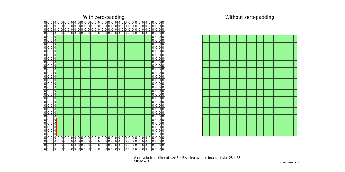
我們可以看到，如果沒有用零填充，則不包括最後四個單元格，因為卷積濾波器已經到達（非零填充）影象的末尾。這意味著，對於28 x 28的輸入大小，輸出大小變為24 x 24 。如果 padding = 'SAME'，則輸出大小為28 x 28。

如果在掃描影象時記下過濾器在影象上的位置（為簡單起見，只有X方向），那麼這一點就變得更加清晰了。如果步幅為1，則X位置為0-5、1-6、2-7，等等。如果步幅為2，則X位置為0-5、2-7、4-9，等等。

如果影象大小為28 x 28，濾鏡大小為5 x 5，並且步長1到4，那麼我們可以得到下面這個表：

可以看到，對於步幅為1，零填充輸出影象大小為28 x 28。如果非零填充，則輸出影象大小變為24 x 24。對於步幅為2的過濾器，這幾個數字分別為 14 x 14 和 12 x 12，對於步幅為3的過濾器，分別為 10 x 10 和 8 x 8。以此類推。

對於任意一個步幅S，濾波器尺寸K，影象尺寸W和填充尺寸P，輸出尺寸將為

如果在Tensorflow中 padding = “SAME”，則分子加起來恆等於1，輸出大小僅由步幅S決定。

2.7 調整 LeNet5 的架構

在原始論文中，LeNet5架構使用了S形啟用函式和平均池。 然而，現在，使用relu啟用函式則更為常見。 所以，我們來稍稍修改一下LeNet5 CNN，看看是否能夠提高準確性。我們將稱之為類LeNet5架構：

LENET5_LIKE_BATCH_SIZE = 32
LENET5_LIKE_FILTER_SIZE = 5
LENET5_LIKE_FILTER_DEPTH = 16
LENET5_LIKE_NUM_HIDDEN = 120

def variables_lenet5_like(filter_size = LENET5_LIKE_FILTER_SIZE, 
                          filter_depth = LENET5_LIKE_FILTER_DEPTH, 
                          num_hidden = LENET5_LIKE_NUM_HIDDEN,
                          image_width = 28, image_depth = 1, num_labels = 10):
 
    w1 = tf.Variable(tf.truncated_normal([filter_size, filter_size, image_depth, filter_depth], stddev=0.1))
    b1 = tf.Variable(tf.zeros([filter_depth]))

    w2 = tf.Variable(tf.truncated_normal([filter_size, filter_size, filter_depth, filter_depth], stddev=0.1))
    b2 = tf.Variable(tf.constant(1.0, shape=[filter_depth]))
 
    w3 = tf.Variable(tf.truncated_normal([(image_width // 4)*(image_width // 4)*filter_depth , num_hidden], stddev=0.1))
    b3 = tf.Variable(tf.constant(1.0, shape = [num_hidden]))

    w4 = tf.Variable(tf.truncated_normal([num_hidden, num_hidden], stddev=0.1))
    b4 = tf.Variable(tf.constant(1.0, shape = [num_hidden]))
 
    w5 = tf.Variable(tf.truncated_normal([num_hidden, num_labels], stddev=0.1))
    b5 = tf.Variable(tf.constant(1.0, shape = [num_labels]))
    variables = {
                  'w1': w1, 'w2': w2, 'w3': w3, 'w4': w4, 'w5': w5,
                  'b1': b1, 'b2': b2, 'b3': b3, 'b4': b4, 'b5': b5
                }
    return variables

def model_lenet5_like(data, variables):
    layer1_conv = tf.nn.conv2d(data, variables['w1'], [1, 1, 1, 1], padding='SAME')
    layer1_actv = tf.nn.relu(layer1_conv + variables['b1'])
    layer1_pool = tf.nn.avg_pool(layer1_actv, [1, 2, 2, 1], [1, 2, 2, 1], padding='SAME')

    layer2_conv = tf.nn.conv2d(layer1_pool, variables['w2'], [1, 1, 1, 1], padding='SAME')
    layer2_actv = tf.nn.relu(layer2_conv + variables['b2'])
    layer2_pool = tf.nn.avg_pool(layer2_actv, [1, 2, 2, 1], [1, 2, 2, 1], padding='SAME')
 
    flat_layer = flatten_tf_array(layer2_pool)
    layer3_fccd = tf.matmul(flat_layer, variables['w3']) + variables['b3']
    layer3_actv = tf.nn.relu(layer3_fccd)
    #layer3_drop = tf.nn.dropout(layer3_actv, 0.5)
 
    layer4_fccd = tf.matmul(layer3_actv, variables['w4']) + variables['b4']
    layer4_actv = tf.nn.relu(layer4_fccd)
   #layer4_drop = tf.nn.dropout(layer4_actv, 0.5)
 
    logits = tf.matmul(layer4_actv, variables['w5']) + variables['b5']
    return logits

主要區別是我們使用了relu啟用函式而不是S形啟用函式。

除了啟用函式，我們還可以改變使用的優化器，看看不同的優化器對精度的影響。

2.8 學習速率和優化器的影響

讓我們來看看這些CNN在MNIST和CIFAR-10資料集上的表現。

在上面的圖中，測試集的精度是迭代次數的函式。左側為一層完全連線的NN，中間為LeNet5 NN，右側為類LeNet5 NN。

可以看到，LeNet5 CNN在MNIST資料集上表現得非常好。這並不是一個大驚喜，因為它專門就是為分類手寫數字而設計的。MNIST資料集很小，並沒有太大的挑戰性，所以即使是一個完全連線的網路也表現的很好。

然而，在CIFAR-10資料集上，LeNet5 NN的效能顯著下降，精度下降到了40％左右。

為了提高精度，我們可以通過應用正則化或學習速率衰減來改變優化器，或者微調神經網路。

可以看到，AdagradOptimizer、AdamOptimizer和RMSPropOptimizer的效能比GradientDescentOptimizer更好。這些都是自適應優化器，其效能通常比GradientDescentOptimizer更好，但需要更多的計算能力。

通過L2正則化或指數速率衰減，我們可能會得到更搞的準確性，但是要獲得更好的結果，我們需要進一步研究。

3. Tensorflow 中的深度神經網路

到目前為止，我們已經看到了LeNet5 CNN架構。 LeNet5包含兩個卷積層，緊接著的是完全連線的層，因此可以稱為淺層神經網路。那時候（1998年），GPU還沒有被用來進行計算，而且CPU的功能也沒有那麼強大，所以，在當時，兩個卷積層已經算是相當具有創新意義了。

後來，很多其他型別的卷積神經網路被設計出來，你可以在這裡檢視詳細資訊。

比如，由Alex Krizhevsky開發的非常有名的AlexNet 架構（2012年），7層的ZF Net (2013)，以及16層的 VGGNet (2014)。

在2015年，Google釋出了一個包含初始模組的22層的CNN（GoogLeNet），而微軟亞洲研究院構建了一個152層的CNN，被稱為ResNet。

現在，根據我們目前已經學到的知識，我們來看一下如何在Tensorflow中建立AlexNet和VGGNet16架構。

3.1 AlexNet

雖然LeNet5是第一個ConvNet，但它被認為是一個淺層神經網路。它在由大小為28 x 28的灰度影象組成的MNIST資料集上執行良好，但是當我們嘗試分類更大、解析度更好、類別更多的影象時，效能就會下降。

第一個深度CNN於2012年推出，稱為AlexNet，其創始人為Alex Krizhevsky、Ilya Sutskever和Geoffrey Hinton。與最近的架構相比，AlexNet可以算是簡單的了，但在當時它確實非常成功。它以令人難以置信的15.4％的測試錯誤率贏得了ImageNet比賽（亞軍的誤差為26.2％），並在全球深度學習和人工智慧領域掀起了一場革命。

它包括5個卷積層、3個最大池化層、3個完全連線層和2個丟棄層。整體架構如下所示：

• 第0層：大小為224 x 224 x 3的輸入影象

• 第1層：具有96個濾波器（filter_depth_1 = 96）的卷積層，大小為11×11（filter_size_1 = 11），步長為4。它包含ReLU啟用函式。

  緊接著的是最大池化層和本地響應歸一化層。

• 第2層：具有大小為5 x 5（filter_size_2 = 5）的256個濾波器（filter_depth_2 = 256）且步幅為1的卷積層。它包含ReLU啟用函式。

  緊接著的還是最大池化層和本地響應歸一化層。

• 第3層：具有384個濾波器的卷積層（filter_depth_3 = 384），尺寸為3×3（filter_size_3 = 3），步幅為1。它包含ReLU啟用函式
• 第4層：與第3層相同。
• 第5層：具有大小為3×3（filter_size_4 = 3）的256個濾波器（filter_depth_4 = 256）且步幅為1的卷積層。它包含ReLU啟用函式
• 第6-8層：這些卷積層之後是完全連線層，每個層具有4096個神經元。在原始論文中，他們對1000個類別的資料集進行分類，但是我們將使用具有17個不同類別（的花卉）的oxford17資料集。