
【深度學習】基於im2col的展開Python實現卷積層和池化層
阿新 • • 發佈:2018-11-26
一、回顧
上一篇 我們介紹了,卷積神經網的卷積計算和池化計算,計算過程中視窗一直在移動,那麼我們如何準確的取到視窗內的元素,並進行正確的計算呢?
另外,以上我們只考慮的單個輸入資料,如果是批量資料呢?
首先,我們先來看看批量資料,是如何計算的
二、批處理
在神經網路的處理中,我們一般將輸入資料進行打包批處理,通過批處理,能夠實現處理的高效化和學習時對mini-batch的對應
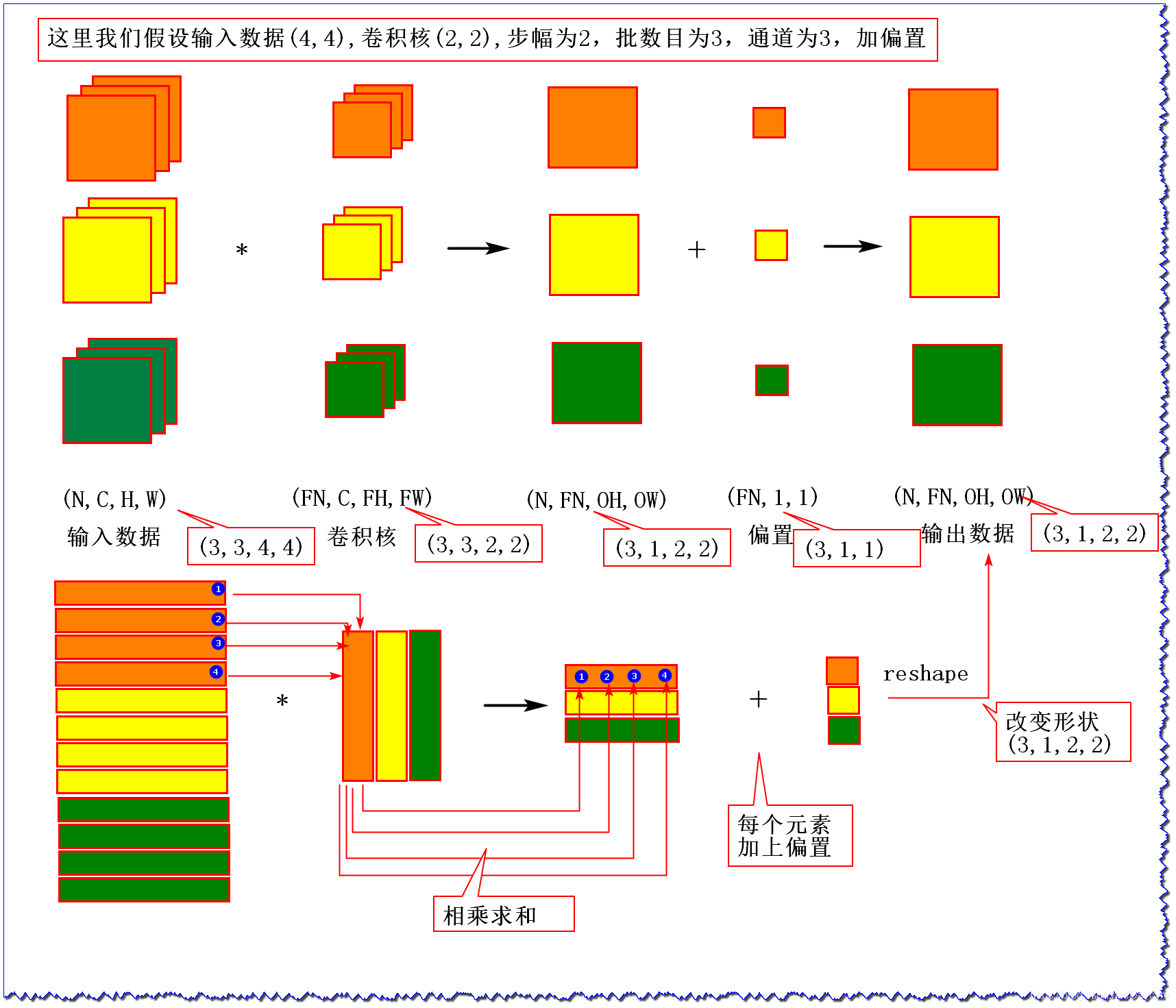
自然,我們也希望在卷積神經網路的卷積運算中也使用批處理,為此,需要將在各層間傳遞的資料儲存為四維資料
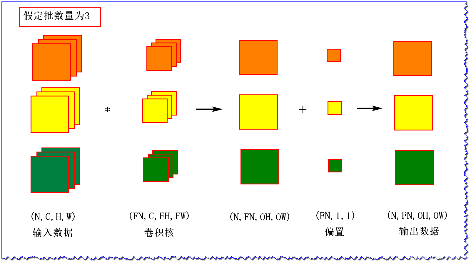
如上圖
- 輸入資料:批數目為3,通道為3
- 卷積核:數目為3,通道為3
- 輸出資料:數目為3,通道為1
三、四維資料
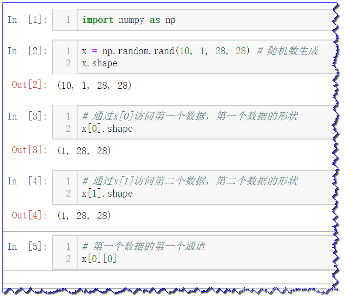
如上所述,CNN中各層將傳遞的資料是四維資料,例如:
- 資料形狀為(10,1,28,28),表示10個高為28,長為28,通道為1的資料
CNN中處理四維資料,按照以上的操作會很複雜,但是通過im2col這個技巧,就會變得很簡單
四、im2col
- 對於輸入資料
- 對於卷積核
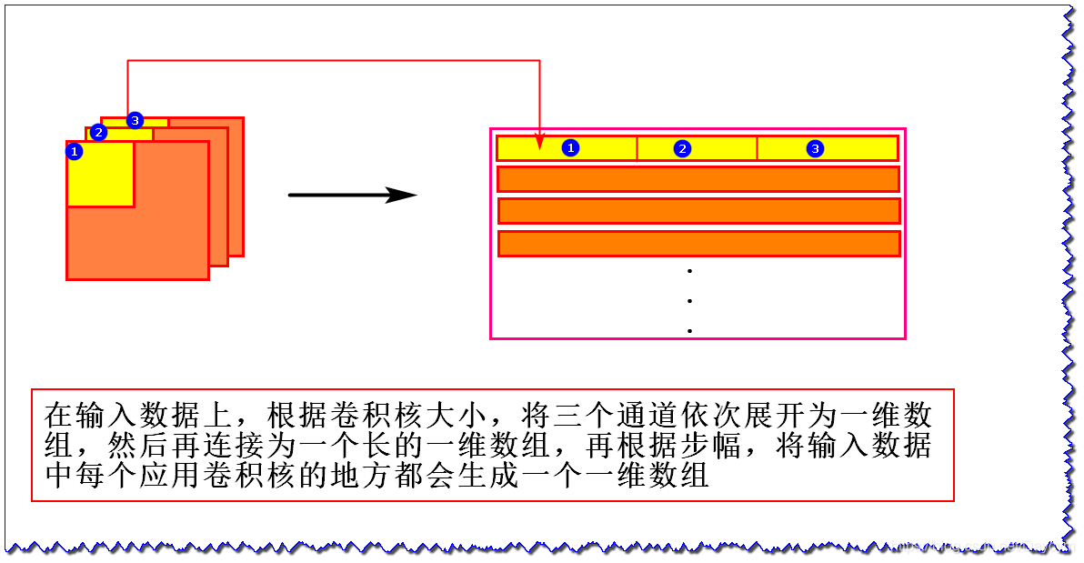
輸入資料展開以適合卷積核(權重)
- 輸入資料,將應用卷積核的區域(3維資料)橫向展開為一行
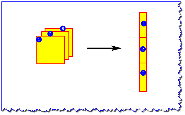
- 卷積核,縱向展開為1列
- 計算乘積即可
- 批量計算
五、python實現im2col和col2im
- np.pad()函式
import numpy as np

A = np.arange(1,5).reshape(2,2)  # 將1,2,3,4轉換為2*2的矩陣
print(A)

B = np.pad(A,((1,1),(2,2)),'constant')
# ((1,1),(2,2))
# 對A矩陣進行擴充,(1,1)表示上下各加一行,(2,2)左右各加兩列
print(B)
輸出為:
[[1 2]
 [3 4]]

[[0 0 0 0 0 0]
 [0 0 1 2 0 0]
 [0 0 3 4 0 0]
 [0 0 0 0 0 0]]
1、im2col
import numpy as np

def im2col(input_data, filter_h, filter_w, stride=1, pad=0):
    """
    Parameters
    ----------
    input_data : 由(資料量, 通道, 高, 長)的4維陣列構成的輸入資料
    filter_h : 卷積核的高
    filter_w : 卷積核的長
    stride : 步幅
    pad : 填充

    Returns
    -------
    col : 2維陣列
    """
    # 輸入資料的形狀
    # N:批數目,C:通道數,H:輸入資料高,W:輸入資料長
    N, C, H, W = input_data.shape
    out_h = (H + 2*pad - filter_h)//stride + 1  # 輸出資料的高
    out_w = (W + 2*pad - filter_w)//stride + 1  # 輸出資料的長
    # 填充 H,W
    img = np.pad(input_data, [(0,0), (0,0), (pad, pad), (pad, pad)], 'constant')
    # (N, C, filter_h, filter_w, out_h, out_w)的0矩陣
    col = np.zeros((N, C, filter_h, filter_w, out_h, out_w))

    for y in range(filter_h):
        y_max = y + stride*out_h
        for x in range(filter_w):
            x_max = x + stride*out_w
            col[:, :, y, x, :, :] = img[:, :, y:y_max:stride, x:x_max:stride]
    # 按(0, 4, 5, 1, 2, 3)順序,交換col的列,然後改變形狀
    col = col.transpose(0, 4, 5, 1, 2, 3).reshape(N*out_h*out_w, -1)
    return col

# 測試
x = np.random.rand(3, 3, 4, 4) # 隨機數生成
print(im2col(x,2,2,2,0))
print(im2col(x,2,2,2,0).shape)
輸出為:
[[0.8126537  0.0124403  0.98329453 0.57534957 0.01075175 0.28476833 0.55240652 0.71247792 0.8866451  0.08312604 0.82491841 0.53558742]
 [0.29177981 0.50891739 0.58534285 0.18979016 0.82281101 0.82324137 0.56737161 0.31075336 0.02638588 0.63497472 0.32696265 0.96400363]
 [0.18770887 0.80279488 0.80743415 0.01885739 0.6043541  0.1325915 0.99802281 0.70238769 0.03320778 0.21225932 0.73413182 0.68671415]
 [0.63299868 0.71823646 0.81703541 0.20652069 0.05803092 0.78660436 0.86116481 0.24152935 0.75596431 0.97947061 0.84386563 0.53657106]
 [0.77410888 0.92973798 0.42845759 0.20494453 0.55320755 0.86069213 0.14749488 0.5110566  0.19249778 0.38564893 0.78868462 0.49548582]
 [0.28778559 0.67286705 0.6351968  0.50743453 0.42905218 0.20382354 0.04566382 0.32610886 0.60199126 0.21139752 0.06912991 0.69890244]
 [0.03473951 0.67443498 0.53320896 0.44542062 0.96787968 0.92660522 0.8726162  0.54056736 0.62510367 0.12935292 0.35858458 0.88899527]
 [0.08295843 0.86116853 0.11507337 0.27507467 0.43662151 0.23341227 0.66133038 0.32065362 0.07386012 0.45717299 0.00857706 0.26429706]
 [0.5203922  0.79072121 0.0861702  0.64400793 0.76287695 0.53397396 0.61997931 0.88647105 0.07416818 0.23701745 0.91067976 0.14036269]
 [0.92652241 0.90052592 0.28945134 0.10758509 0.66142524 0.81998174 0.29023353 0.10070337 0.84680753 0.38787205 0.62224245 0.25184519]
 [0.00896273 0.86085848 0.72448385 0.97710942 0.27221302 0.30631167 0.80608232 0.92652234 0.35904511 0.26833127 0.72821478 0.72382557]
 [0.31399633 0.12624691 0.37392867 0.71121627 0.98641763 0.01551433 0.82284883 0.67615753 0.21826556 0.90338993 0.41159445 0.98961608]]
(12, 12)
我們設定如上圖中的形狀
- 輸入資料:(3,3,4,4)
- 卷積核:(2,2)
- 結果為:(12,12)
結果和圖中的結果一樣,12行(3個數據,每個資料4行),每行有12個元素(應用(2,2)卷積核1次,三個通道,322=12)
2、col2im
def col2im(col, input_shape, filter_h, filter_w, stride=1, pad=0):
    N, C, H, W = input_shape
    out_h = (H + 2*pad - filter_h)//stride + 1
    out_w = (W + 2*pad - filter_w)//stride + 1
    col = col.reshape(N, out_h, out_w, C, filter_h, filter_w).transpose(0, 3, 4, 5, 1, 2)

    img = np.zeros((N, C, H + 2*pad + stride - 1, W + 2*pad + stride - 1))
    for y in range(filter_h):
        y_max = y + stride*out_h
        for x in range(filter_w):
            x_max = x + stride*out_w
            img[:, :, y:y_max:stride, x:x_max:stride] += col[:, :, y, x, :, :]

    return img[:, :, pad:H + pad, pad:W + pad]
六、實現卷積層
class Convolution:
	# 初始化權重(卷積核4維)、偏置、步幅、填充
    def __init__(self, W, b, stride=1, pad=0):
        self.W = W
        self.b = b
        self.stride = stride
        self.pad = pad

        # 中間資料(backward時使用)
        self.x = None
        self.col = None
        self.col_W = None

        # 權重和偏置引數的梯度
        self.dW = None
        self.db = None

    def forward(self, x):
        # 卷積核大小
        FN, C, FH, FW = self.W.shape
        # 資料資料大小
        N, C, H, W = x.shape
        # 計算輸出資料大小
        out_h = 1 + int((H + 2*self.pad - FH) / self.stride)
        out_w = 1 + int((W + 2*self.pad - FW) / self.stride)
        # 利用im2col轉換為行
        col = im2col(x, FH, FW, self.stride, self.pad)
        # 卷積核轉換為列,展開為2維陣列
        col_W = self.W.reshape(FN, -1).T
        # 計算正向傳播
        out = np.dot(col, col_W) + self.b
        out = out.reshape(N, out_h, out_w, -1).transpose(0, 3, 1, 2)

        self.x = x
        self.col = col
        self.col_W = col_W

        return out

    def backward(self, dout):
        # 卷積核大小
        FN, C, FH, FW = self.W.shape
        dout = dout.transpose(0,2,3,1).reshape(-1, FN)

        self.db = np.sum(dout, axis=0)
        self.dW = np.dot(self.col.T, dout)
        self.dW = self.dW.transpose(1, 0).reshape(FN, C, FH, FW)

        dcol = np.dot(dout, self.col_W.T)
        # 逆轉換
        dx = col2im(dcol, self.x.shape, FH, FW, self.stride, self.pad)

        return dx
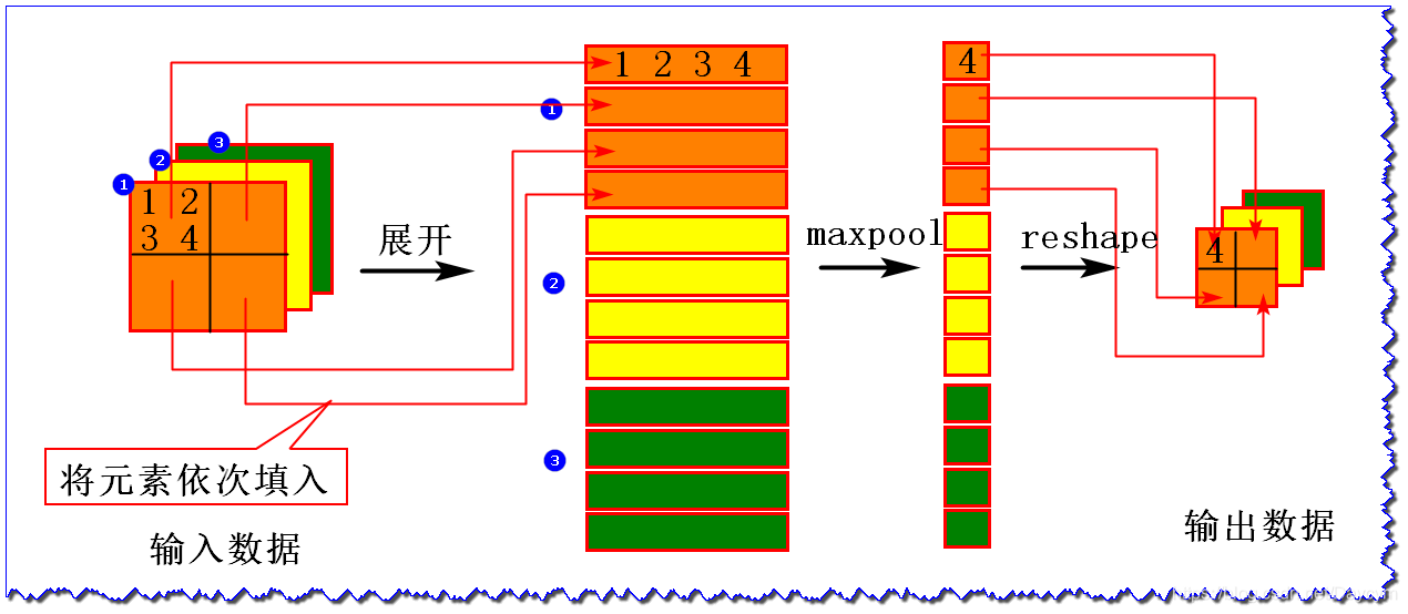
七、實現池化層
class Pooling:
    def __init__(self, pool_h, pool_w, stride=1, pad=0):
        self.pool_h = pool_h
        self.pool_w = pool_w
        self.stride = stride
        self.pad = pad

        self.x = None
        self.arg_max = None

    def forward(self, x):
        N, C, H, W = x.shape
        out_h = int(1 + (H - self.pool_h) / self.stride)
        out_w = int(1 + (W - self.pool_w) / self.stride)
		# 展開
        col = im2col(x, self.pool_h, self.pool_w, self.stride, self.pad)
        col = col.reshape(-1, self.pool_h*self.pool_w)
		# 最大值
        arg_max = np.argmax(col, axis=1)
        out = np.max(col, axis=1)
        # 轉換
        out = out.reshape(N, out_h, out_w, C).transpose(0, 3, 1, 2)

        self.x = x
        self.arg_max = arg_max

        return out

    def backward(self, dout):
        dout = dout.transpose(0, 2, 3, 1)

        pool_size = self.pool_h * self.pool_w
        dmax = np.zeros((dout.size, pool_size))
        dmax[np.arange(self.arg_max.size), self.arg_max.flatten()] = dout.flatten()
        dmax = dmax.reshape(dout.shape + (pool_size,))

        dcol = dmax.reshape(dmax.shape[0] * dmax.shape[1] * dmax.shape[2], -1)
        dx = col2im(dcol, self.x.shape, self.pool_h, self.pool_w, self.stride, self.pad)

        return dx
總結
- 本篇的難點在於資料的展開和逆轉換
- 關於卷積層和池化層的計算也比較好理解,但是程式碼實現有點繞,不過原理和神經網路中的全連線層實現方式一樣