基準資料集

深度學習中經常會使用一些基準資料集進行一些測試。其中 MNIST, Cifar 10, cifar100, Fashion-MNIST 資料集常常被人們拿來當作練手的資料集。為了方便，諸如 Keras、MXNet、Tensorflow 都封裝了自己的基礎資料集，如 MNIST、cifar 等。如果我們要在不同平臺使用這些資料集，還需要了解那些框架是如何組織這些資料集的，需要花費一些不必要的時間學習它們的 API。為此，我們為何不建立屬於自己的資料集呢？下面我僅僅使用了 Numpy 來實現資料集 MNIST、Fashion MNIST

、Cifa 10、Cifar 100 的操作，並封裝為 HDF5，這樣該資料集的可擴充套件性就會大大的增強，並且還可以被其他的程式語言 (如 Matlab) 來獲取和使用。下面主要介紹如何通過建立的 API 來實現資料集的封裝。

環境搭建

我使用了 Anaconda3 這個十分好用的包管理工具, 來減少管理和安裝一些必須的包。下面我們載入該 API 必備的包：

import struct   # 處理二進位制檔案
import numpy as np   # 對矩陣運算很友好
import gzip, tarfile  # 對壓縮檔案進行處理
import os          # 管理本地檔案
import pickle      # 序列化和反序列化
import time       # 記時
 

我是在 Jupyter Notebook 互動環境中執行程式碼的。

Bunch 結構

為了更好的使用該 API, 我利用了 Bunch 結構。在 Python 中，我們可以定義 Bunch Pattern, 字面意思大概是指鏈式的束式結構。主要用於儲存鬆散的資料結構。

它能讓我們以命令列引數的形式建立相關物件，並設定任何屬性。下面我們來看看 Bunch 的魅力！Bunch 的定義利用了 dict 的特性。

class Bunch(dict):
    
    def __init__(self, *args, **kwds):
        super().__init__(*args, **kwds)
        self.__dict__ = self
 

下面我們構建一個 Bunch 的例項 Tom, 它代表一個住在北京的 54 歲的人。

Tom = Bunch(age="54", address="Beijing")

我們可以檢視 Tom 的一些資訊：

print('Tom 的年齡是 {}，他住在 {}.'.format(Tom.age, Tom.address))

Tom 的年齡是 54，他住在 Beijing.

我們還可以直接對 Tom 增加屬性，比如：

Tom.sex = 'male'
print(Tom)

{'age': '54', 'address': 'Beijing', 'sex': 'male'}

你也許會奇怪，Bunch 結構與 dict 結構好像沒有太大的的區別，只不過是多了一個點號運算，那麼，Bunch 到底有什麼神奇之處呢？我們先看一個例子：

T = Bunch
t = T(left=T(left='a',right='b'), right=T(left='c'))

for first in t:
    print('第一層的節點：', first)
    for second in t[first]:
        print('\t第二層的節點：', second)
        for node in t[first][second]:
            print('\t\t第三層的節點：', node)

第一層的節點： left
    第二層的節點： left
        第三層的節點： a
    第二層的節點： right
        第三層的節點： b
第一層的節點： right
    第二層的節點： left
        第三層的節點： c

從上面的輸出我們可以看出，t 便是一個簡單的二叉樹結構。這樣，我們便可使用 Bunch 構建許多具有分層結構的資料型別。

下載資料集

連結：

• MNIST: http://yann.lecun.com/exdb/mnist
• Fashion MNIST: https://github.com/zalandoresearch/fashion-mnist
• Cifar: https://www.cs.toronto.edu/~kriz/cifar.html

我們將上述資料集均下載到同一個目錄下，比如：'E:/Data/Zip/'，下面我們將逐一介紹上述資料集。

MNIST & Fashion MNIST

MNIST 資料集可以說是深度學習中的 hello world 級別的資料集，很多教程都是把它作為入門級的資料集。不過有些人可能對它還不是很瞭解, 下面我們簡單的瞭解一下！

MNIST 資料集來自美國國家標準與技術研究所（National Institute of Standards and Technology, NIST）. 訓練集 (training set) 由來自 250 個不同人手寫的數字構成, 其中 50%50% 是高中學生, 50%50% 來自人口普查局 (the Census Bureau) 的工作人員. 測試集(test set) 也是同樣比例的手寫數字資料.

MNIST 有一組 6000060000 個樣本的訓練集和一組 1000010000 個樣本的測試集。它是 NIST 的子集。數字影象已被大小規範化, 並以固定大小的影象居中。

MNIST 資料集可在 http://yann.lecun.com/exdb/mnist/ 獲取, 它包含了四個部分:

• train-images-idx3-ubyte.gz: training set images (9912422 bytes)
• train-labels-idx1-ubyte.gz: training set labels (28881 bytes)
• t10k-images-idx3-ubyte.gz: test set images (1648877 bytes)
• t10k-labels-idx1-ubyte.gz: test set labels (4542 bytes)

影象分類資料集中最常用的是手寫數字識別資料集 MNIST1。但大部分模型在 MNIST 上的分類精度都超過了 95%95%。為了更直觀地觀察演算法之間的差異，我們可以使用一個影象內容更加複雜的資料集 Fashion-MNIST2。Fashion-MNIST 和 MNIST 一樣，也包括了 1010 個類別，分別為：t-shirt（T 恤）、trouser（褲子）、pullover（套衫）、dress（連衣裙）、coat（外套）、sandal（涼鞋）、shirt（襯衫）、sneaker（運動鞋）、bag（包）和 ankle boot（短靴）。

Fashion-MNIST 的儲存方式和 MNIST 是一樣的，故而，我們可以使用相同的方式對其進行處理。

MNIST 的使用

下面我以 MNIST 類來處理 MNIST 和 Fashion MNIST:

class MNIST:
    def __init__(self, root, namespace, train=True, transform=None):
        """
        (MNIST handwritten digits dataset from http://yann.lecun.com/exdb/mnist)
        (A dataset of Zalando's article images consisting of fashion products,
        a drop-in replacement of the original MNIST dataset
        from https://github.com/zalandoresearch/fashion-mnist)

        Each sample is an image (in 3D NDArray) with shape (28, 28, 1).

        Parameters
        ----------
        root : 資料根目錄，如 'E:/Data/Zip/'
        namespace : 'mnist' or 'fashion_mnist'
        train : bool, default True
            Whether to load the training or testing set.
        transform : function, default None
            A user defined callback that transforms each sample. For example:
        ::

            transform=lambda data, label: (data.astype(np.float32)/255, label)
        """
        self._train = train
        self.namespace = namespace
        root = root + namespace
        self._train_data = f'{root}/train-images-idx3-ubyte.gz'
        self._train_label = f'{root}/train-labels-idx1-ubyte.gz'
        self._test_data = f'{root}/t10k-images-idx3-ubyte.gz'
        self._test_label = f'{root}/t10k-labels-idx1-ubyte.gz'
        self._get_data()

    def _get_data(self):
        '''
        官方網站的資料是以 `[offset][type][value][description]` 的格式封裝的，
        因而 `struct.unpack` 時需要注意
        '''
        if self._train:
            data, label = self._train_data, self._train_label
        else:
            data, label = self._test_data, self._test_label

        with gzip.open(label, 'rb') as fin:
            struct.unpack(">II", fin.read(8))
            self.label = np.frombuffer(fin.read(), dtype=np.uint8)

        with gzip.open(data, 'rb') as fin:
            Y = struct.unpack(">IIII", fin.read(16))
            data = np.frombuffer(fin.read(), dtype=np.uint8)
            self.data = data.reshape(Y[1:])

下面，我們來看看如何載入這兩個資料集？

MNIST

考慮到程式碼的可複用性，我將上述程式碼封裝在我的 GitHub3
。將其下載到本地，你便可以直接使用。下面我將展示如何使用該 API。

首先，需要找到你下載的 API 目錄，比如：D:\GitHub\basedataset\loader，然後載入到你當前的 Python 環境變數中。

import sys

sys.path.append('D:/GitHub/basedataset/loader/')

from zdata import MNIST

下面你便可以自如的呼叫 MNIST 類了。

root = 'E:/Data/Zip/'
namespace = 'mnist'
train_mnist = MNIST(root, namespace, train=True, transform=None)  # 獲取訓練集
test_mnist = MNIST(root, namespace, train=False, transform=None)  # 獲取測試集

print('MNIST 的訓練集規模：{}'.format((train_mnist.data.shape)))
print('MNIST 的測試集規模：{}'.format((test_mnist.data.shape)))

MNIST 的訓練集規模：(60000, 28, 28)
MNIST 的測試集規模：(10000, 28, 28)

下面我們以 MNIST 的測試集為例，來看看 MNIST 具體長什麼樣吧！

from matplotlib import pyplot as plt


def show_imgs(imgs):
    '''
    展示 多張圖片
    '''
    n = imgs.shape[0]
    h, w = 4, int(n / 4)
    _, figs = plt.subplots(h, w, figsize=(5, 5))
    K = np.arange(n).reshape((h, w))
    for i in range(h):
        for j in range(w):
            img = imgs[K[i, j]]
            figs[i][j].imshow(img)
            figs[i][j].axes.get_xaxis().set_visible(False)
            figs[i][j].axes.get_yaxis().set_visible(False)
    plt.show()

imgs = test_mnist.data[:16]
show_imgs(imgs)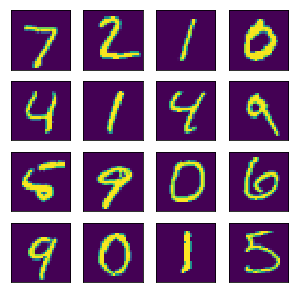

Fashion MNIST

namespace = 'fashion_mnist'
train_mnist_f = MNIST(root, namespace, train=True, transform=None)
test_mnist_f = MNIST(root, namespace, train=False, transform=None)

print('Fashion MNIST 的訓練集規模：{}'.format((train_mnist_f.data.shape)))
print('Fashion MNIST 的測試集規模：{}'.format((test_mnist_f.data.shape)))

Fashion MNIST 的訓練集規模：(60000, 28, 28)
Fashion MNIST 的測試集規模：(10000, 28, 28)

再看看 Fashion MNIST 具體長什麼樣吧！

imgs_f = test_mnist_f.data[:16]
show_imgs(imgs_f)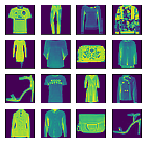

MNIST 和 Fashion MNIST 資料集還是太簡單了，為了滿足更多的需求，下面我們將進入 Cifar 資料集的 API 開發和使用環節。

Cifar API

class Bunch(dict):
    def __init__(self, *args, **kwds):
        super().__init__(*args, **kwds)
        self.__dict__ = self


class Cifar(Bunch):
    def __init__(self, root, namespace, transform=None, *args, **kwds):
        """CIFAR image classification dataset
         from https://www.cs.toronto.edu/~kriz/cifar.html

        Each sample is an image (in 3D NDArray) with shape (32, 32, 3).

        Parameters
        ----------
        meta : 儲存了類別資訊
        root : str, 資料根目錄
        namespace : 'cifar-10' 或 'cifar-100'
        transform : function, default None
            A user defined callback that transforms each sample. For example:
        ::

            transform=lambda data, label: (data.astype(np.float32)/255, label)

        """
        super().__init__(*args, **kwds)
        self.url = 'https://www.cs.toronto.edu/~kriz/cifar.html'
        self.namespace = namespace
        self._extract(root)
        self._read_batch()

    def _extract(self, root):
        tar_name = f'{root}{self.namespace}-python.tar.gz'
        names = extractall(tar_name, root)
        # print('載入資料的字典資訊：')
        #start = time.time()
        for name in names:
            path = f'{root}{name}'

            if os.path.isfile(path):
                if not (path.endswith('.html') or path.endswith('.txt~')):
                    k = name.split('/')[-1]
                    if path.endswith('meta'):
                        with open(path, 'rb') as fp:
                            self['meta'] = pickle.load(fp)
                    else:
                        with open(path, 'rb') as fp:
                            self[k] = pickle.load(fp, encoding='bytes')

        #     #time.sleep(0.2)
        #     t = int(time.time() - start) * '-'
        #     print(t, end='')
        # print('\n載入資料的字典資訊完畢！')

    def _read_batch(self):
        if self.namespace == 'cifar-10':
            self.trainX = np.concatenate([
                self[f'data_batch_{str(i)}'][b'data'] for i in range(1, 6)
            ]).reshape(-1, 3, 32, 32).transpose((0, 2, 3, 1))
            self.trainY = np.concatenate([
                np.asanyarray(self[f'data_batch_{str(i)}'][b'labels'])
                for i in range(1, 6)
            ])
            self.testX = self.test_batch[b'data'].reshape(
                -1, 3, 32, 32).transpose((0, 2, 3, 1))
            self.testY = np.asanyarray(self.test_batch[b'labels'])
        elif self.namespace == 'cifar-100':
            self.trainX = self.train[b'data'].reshape(-1, 3, 32, 32)
            self.train_fine_labels = np.asanyarray(
                self.train[b'fine_labels'])  # 子類標籤
            self.train_coarse_labels = np.asanyarray(
                self.train[b'coarse_labels'])  # 超類標籤
            self.testX = self.test[b'data'].reshape(-1, 3, 32, 32)
            self.test_fine_labels = np.asanyarray(
                self.test[b'fine_labels'])  # 子類標籤
            self.test_coarse_labels = np.asanyarray(
                self.test[b'coarse_labels'])  # 超類標籤

為了方便管理和呼叫資料集，我定義了一個 DataBunch 類：

class DataBunch(Bunch):
    '''
    將資料集轉換為 Bunch
    '''
    def __init__(self, root, *args, **kwds):
        super().__init__(*args, **kwds)
        B = Bunch
        self.mnist = B(MNIST(root, 'mnist'))
        self.fashion_mnist = B(MNIST(root, 'fashion_mnist'))
        self.cifar10 = B(Cifar(root, 'cifar-10'))
        self.cifar100 = B(Cifar(root, 'cifar-100'))

同樣將上述程式碼放入 zdata 模組中。

Cifar 10 資料集

下面我們便可以直接利用 DataBunch 類來呼叫上述介紹的資料集：

import sys

sys.path.append('D:/GitHub/basedataset/loader/')

from zdata import DataBunch, show_imgs

root = 'E:/Data/Zip/'
db = DataBunch(root)

我們可以檢視，我們封裝的資料集：

db.keys()

dict_keys(['mnist', 'fashion_mnist', 'cifar10', 'cifar100'])

由於前面已經展示過 'mnist', 'fashion_mnist'，下面我們將展示 Cifar API 的使用。更多詳細內容參考我的博文 關於 『AI 專屬資料庫的定製』的改進4。

cifar-10 和 CIFAR-10 標記為 80008000 萬個 微小影象資料集5的子集。它們是由 Alex Krizhevsky, Vinod Nair, 和 Geoffrey Hinton 收集的。

cifar-10 資料集由 1010 類 32×3232×32 彩色影象組成, 每類有 60006000 張影象。被劃分為 5000050000 張訓練影象和 1000010000 張測試影象。

cifar10 = db.cifar10

imgs = cifar10.trainX[:16]
show_imgs(imgs)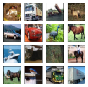

為了方便資料的使用，我們可以將 db 寫入到本地磁碟：

序列化

import pickle

def write_bunch(path):
    '''
    path:: 寫入資料集的檔案路徑
    '''
    with open(path, 'wb') as fp:
        pickle.dump(db, fp)

root = 'E:/Data/Zip/'
path = f'{root}X.json'   # 寫入資料集的檔案路徑
write_bunch(path)

這樣以後我們就可以直接複製 f'{root}X.dat 或 f'{root}X.json' 到你可以放置的任何地方，然後你就可以通過 load 函式來呼叫 MNIST、Fashion MNIST、Cifa 10、Cifar 100 這些資料集。即：

反序列化

def read_bunch(path):
    with open(path, 'rb') as fp:
        bunch = pickle.load(fp)  # 即為上面的 DataBunch 的例項
    return bunch

db = read_bunch(path)   # path 即你的資料集所在的路徑

考慮到 JSON 對於其他程式語言的不友好，下面我們將介紹如何將 Bunch 資料集儲存為 HDF5 格式的資料。

Bunch 轉換為 HDF5 檔案：高效儲存 Cifar 等資料集

PyTables6 是 Python 與 HDF5 資料庫/檔案標準的結合7。它專門為優化 I/O 操作的效能、最大限度地利用可用硬體而設計，並且它還支援壓縮功能。

下面的程式碼均是在 Jupyter NoteBook 下完成的：

import tables as tb
import numpy as np


def bunch2hdf5(root):
    '''
    這裡我僅僅封裝了 Cifar10、Cifar100、MNIST、Fashion MNIST 資料集，
    使用者還可以自己追加資料集。
    '''
    db = DataBunch(root)
    filters = tb.Filters(complevel=7, shuffle=False)
    # 這裡我採用了壓縮表，因而儲存為 `.h5c` 但也可以儲存為 `.h5`
    with tb.open_file(f'{root}X.h5c', 'w', filters=filters, title='Xinet\'s dataset') as h5:
        for name in db.keys():
            h5.create_group('/', name, title=f'{db[name].url}')
            if name != 'cifar100':
                h5.create_array(h5.root[name], 'trainX', db[name].trainX, title='訓練資料')
                h5.create_array(h5.root[name], 'trainY', db[name].trainY, title='訓練標籤')
                h5.create_array(h5.root[name], 'testX', db[name].testX, title='測試資料')
                h5.create_array(h5.root[name], 'testY', db[name].testY, title='測試標籤')
            else:
                h5.create_array(h5.root[name], 'trainX', db[name].trainX, title='訓練資料')
                h5.create_array(h5.root[name], 'testX', db[name].testX, title='測試資料')
                h5.create_array(h5.root[name], 'train_coarse_labels', db[name].train_coarse_labels, title='超類訓練標籤')
                h5.create_array(h5.root[name], 'test_coarse_labels', db[name].test_coarse_labels, title='超類測試標籤')
                h5.create_array(h5.root[name], 'train_fine_labels', db[name].train_fine_labels, title='子類訓練標籤')
                h5.create_array(h5.root[name], 'test_fine_labels', db[name].test_fine_labels, title='子類測試標籤')

        for k in ['cifar10', 'cifar100']:
            for name in db[k].meta.keys():
                name = name.decode()
                if name.endswith('names'):
                    label_names = np.asanyarray([label_name.decode() for label_name in db[k].meta[name.encode()]])
                    h5.create_array(h5.root[k], name, label_names, title='標籤名稱')

完成 Bunch到 HDF5 的轉換

root = 'E:/Data/Zip/'
bunch2hdf5(root)

h5c = tb.open_file('E:/Data/Zip/X.h5c')
h5c

File(filename=E:/Data/Zip/X.h5c, title="Xinet's dataset", mode='r', root_uep='/', filters=Filters(complevel=7, complib='zlib', shuffle=False, bitshuffle=False, fletcher32=False, least_significant_digit=None))
/ (RootGroup) "Xinet's dataset"
/cifar10 (Group) 'https://www.cs.toronto.edu/~kriz/cifar.html'
/cifar10/label_names (Array(10,)) '標籤名稱'
  atom := StringAtom(itemsize=10, shape=(), dflt=b'')
  maindim := 0
  flavor := 'numpy'
  byteorder := 'irrelevant'
  chunkshape := None
/cifar10/testX (Array(10000, 32, 32, 3)) '測試資料'
  atom := UInt8Atom(shape=(), dflt=0)
  maindim := 0
  flavor := 'numpy'
  byteorder := 'irrelevant'
  chunkshape := None
/cifar10/testY (Array(10000,)) '測試標籤'
  atom := Int32Atom(shape=(), dflt=0)
  maindim := 0
  flavor := 'numpy'
  byteorder := 'little'
  chunkshape := None
/cifar10/trainX (Array(50000, 32, 32, 3)) '訓練資料'
  atom := UInt8Atom(shape=(), dflt=0)
  maindim := 0
  flavor := 'numpy'
  byteorder := 'irrelevant'
  chunkshape := None
/cifar10/trainY (Array(50000,)) '訓練標籤'
  atom := Int32Atom(shape=(), dflt=0)
  maindim := 0
  flavor := 'numpy'
  byteorder := 'little'
  chunkshape := None
/cifar100 (Group) 'https://www.cs.toronto.edu/~kriz/cifar.html'
/cifar100/coarse_label_names (Array(20,)) '標籤名稱'
  atom := StringAtom(itemsize=30, shape=(), dflt=b'')
  maindim := 0
  flavor := 'numpy'
  byteorder := 'irrelevant'
  chunkshape := None
/cifar100/fine_label_names (Array(100,)) '標籤名稱'
  atom := StringAtom(itemsize=13, shape=(), dflt=b'')
  maindim := 0
  flavor := 'numpy'
  byteorder := 'irrelevant'
  chunkshape := None
/cifar100/testX (Array(10000, 32, 32, 3)) '測試資料'
  atom := UInt8Atom(shape=(), dflt=0)
  maindim := 0
  flavor := 'numpy'
  byteorder := 'irrelevant'
  chunkshape := None
/cifar100/test_coarse_labels (Array(10000,)) '超類測試標籤'
  atom := Int32Atom(shape=(), dflt=0)
  maindim := 0
  flavor := 'numpy'
  byteorder := 'little'
  chunkshape := None
/cifar100/test_fine_labels (Array(10000,)) '子類測試標籤'
  atom := Int32Atom(shape=(), dflt=0)
  maindim := 0
  flavor := 'numpy'
  byteorder := 'little'
  chunkshape := None
/cifar100/trainX (Array(50000, 32, 32, 3)) '訓練資料'
  atom := UInt8Atom(shape=(), dflt=0)
  maindim := 0
  flavor := 'numpy'
  byteorder := 'irrelevant'
  chunkshape := None
/cifar100/train_coarse_labels (Array(50000,)) '超類訓練標籤'
  atom := Int32Atom(shape=(), dflt=0)
  maindim := 0
  flavor := 'numpy'
  byteorder := 'little'
  chunkshape := None
/cifar100/train_fine_labels (Array(50000,)) '子類訓練標籤'
  atom := Int32Atom(shape=(), dflt=0)
  maindim := 0
  flavor := 'numpy'
  byteorder := 'little'
  chunkshape := None
/fashion_mnist (Group) 'https://github.com/zalandoresearch/fashion-mnist'
/fashion_mnist/testX (Array(10000, 28, 28, 1)) '測試資料'
  atom := UInt8Atom(shape=(), dflt=0)
  maindim := 0
  flavor := 'numpy'
  byteorder := 'irrelevant'
  chunkshape := None
/fashion_mnist/testY (Array(10000,)) '測試標籤'
  atom := Int32Atom(shape=(), dflt=0)
  maindim := 0
  flavor := 'numpy'
  byteorder := 'little'
  chunkshape := None
/fashion_mnist/trainX (Array(60000, 28, 28, 1)) '訓練資料'
  atom := UInt8Atom(shape=(), dflt=0)
  maindim := 0
  flavor := 'numpy'
  byteorder := 'irrelevant'
  chunkshape := None
/fashion_mnist/trainY (Array(60000,)) '訓練標籤'
  atom := Int32Atom(shape=(), dflt=0)
  maindim := 0
  flavor := 'numpy'
  byteorder := 'little'
  chunkshape := None
/mnist (Group) 'http://yann.lecun.com/exdb/mnist'
/mnist/testX (Array(10000, 28, 28, 1)) '測試資料'
  atom := UInt8Atom(shape=(), dflt=0)
  maindim := 0
  flavor := 'numpy'
  byteorder := 'irrelevant'
  chunkshape := None
/mnist/testY (Array(10000,)) '測試標籤'
  atom := Int32Atom(shape=(), dflt=0)
  maindim := 0
  flavor := 'numpy'
  byteorder := 'little'
  chunkshape := None
/mnist/trainX (Array(60000, 28, 28, 1)) '訓練資料'
  atom := UInt8Atom(shape=(), dflt=0)
  maindim := 0
  flavor := 'numpy'
  byteorder := 'irrelevant'
  chunkshape := None
/mnist/trainY (Array(60000,)) '訓練標籤'
  atom := Int32Atom(shape=(), dflt=0)
  maindim := 0
  flavor := 'numpy'
  byteorder := 'little'
  chunkshape := None

從上面的結構可看出我將 Cifar10、Cifar100、MNIST、Fashion MNIST 進行了封裝，並且還附帶了它們各種的資料集資訊。比如標籤名，數字特徵（以陣列的形式進行封裝）等。

%%time
arr = h5c.root.cifar100.trainX.read() # 讀取資料十分快速

Wall time: 125 ms

arr.shape

(50000, 32, 32, 3)

h5c.root

/ (RootGroup) "Xinet's dataset"
  children := ['cifar10' (Group), 'cifar100' (Group), 'fashion_mnist' (Group), 'mnist' (Group)]

X.h5c 使用說明

下面我們以 Cifar100 為例來展示我們自創的資料集 X.h5c（我將其上傳到了百度雲盤「連結：https://pan.baidu.com/s/1hsbMhv3MDlOES3UDDmOQiw 密碼：qlb7」可以下載直接使用；亦可你自己生成，不過我推薦自己生成，可以對資料集加深理解）

cifar100 = h5c.root.cifar100
cifar100

/cifar100 (Group) 'https://www.cs.toronto.edu/~kriz/cifar.html'
  children := ['coarse_label_names' (Array), 'fine_label_names' (Array), 'testX' (Array), 'test_coarse_labels' (Array), 'test_fine_labels' (Array), 'trainX' (Array), 'train_coarse_labels' (Array), 'train_fine_labels' (Array)]

'coarse_label_names' 指的是粗粒度或超類標籤名，'fine_label_names' 則是細粒度標籤名。

可以使用 read() 方法直接獲取資訊，也可以使用索引的方式獲取。

coarse_label_names = cifar100.coarse_label_names[:]
# 或者
coarse_label_names = cifar100.coarse_label_names.read()
coarse_label_names.astype('str')

array(['aquatic_mammals', 'fish', 'flowers', 'food_containers',
       'fruit_and_vegetables', 'household_electrical_devices',
       'household_furniture', 'insects', 'large_carnivores',
       'large_man-made_outdoor_things', 'large_natural_outdoor_scenes',
       'large_omnivores_and_herbivores', 'medium_mammals',
       'non-insect_invertebrates', 'people', 'reptiles', 'small_mammals',
       'trees', 'vehicles_1', 'vehicles_2'], dtype='<U30')

fine_label_names = cifar100.fine_label_names[:].astype('str')
fine_label_names

array(['apple', 'aquarium_fish', 'baby', 'bear', 'beaver', 'bed', 'bee',
       'beetle', 'bicycle', 'bottle', 'bowl', 'boy', 'bridge', 'bus',
       'butterfly', 'camel', 'can', 'castle', 'caterpillar', 'cattle',
       'chair', 'chimpanzee', 'clock', 'cloud', 'cockroach', 'couch',
       'crab', 'crocodile', 'cup', 'dinosaur', 'dolphin', 'elephant',
       'flatfish', 'forest', 'fox', 'girl', 'hamster', 'house',
       'kangaroo', 'keyboard', 'lamp', 'lawn_mower', 'leopard', 'lion',
       'lizard', 'lobster', 'man', 'maple_tree', 'motorcycle', 'mountain',
       'mouse', 'mushroom', 'oak_tree', 'orange', 'orchid', 'otter',
       'palm_tree', 'pear', 'pickup_truck', 'pine_tree', 'plain', 'plate',
       'poppy', 'porcupine', 'possum', 'rabbit', 'raccoon', 'ray', 'road',
       'rocket', 'rose', 'sea', 'seal', 'shark', 'shrew', 'skunk',
       'skyscraper', 'snail', 'snake', 'spider', 'squirrel', 'streetcar',
       'sunflower', 'sweet_pepper', 'table', 'tank', 'telephone',
       'television', 'tiger', 'tractor', 'train', 'trout', 'tulip',
       'turtle', 'wardrobe', 'whale', 'willow_tree', 'wolf', 'woman',
       'worm'], dtype='<U13')

'testX' 與 'trainX' 分別代表資料的測試資料和訓練資料，而其他的節點所代表的含義也是類似的。

例如，我們可以看看訓練集的資料和標籤：

trainX = cifar100.trainX
train_coarse_labels = cifar100.train_coarse_labels

array([11, 15,  4, ...,  8,  7,  1])

shape 為 (50000, 32, 32, 3)，資料的獲取，我們一樣可以採用索引的形式或者使用 read()：

train_data = trainX[:]
print(train_data[0].shape)
print(train_data.dtype)

(32, 32, 3)
uint8

當然，我們也可以直接使用 trainX 做運算。

for x in cifar100.trainX:
    y = x * 2
    break

print(y.shape)

(32, 32, 3)

h5c.get_node(h5c.root.cifar100, 'trainX')

/cifar100/trainX (Array(50000, 32, 32, 3)) '訓練資料'
  atom := UInt8Atom(shape=(), dflt=0)
  maindim := 0
  flavor := 'numpy'
  byteorder := 'irrelevant'
  chunkshape := None

更甚者，我們可以直接定義迭代器來獲取資料：

trainX = cifar100.trainX
train_coarse_labels = cifar100.train_coarse_labels

def data_iter(X, Y, batch_size):
    n = X.nrows
    idx = np.arange(n)
    if X.name.startswith('train'):
        np.random.shuffle(idx)
    for i in range(0, n ,batch_size):
        k = idx[i: min(n, i + batch_size)].tolist()
        yield np.take(X, k, 0), np.take(Y, k, 0)

for x, y in data_iter(trainX, train_coarse_labels, 8):
    print(x.shape, y)
    break

(8, 32, 32, 3) [ 7  7  0 15  4  8  8  3]

更多使用詳情見：使用 迭代器 獲取 Cifar 等常用資料集8

為了更加形象的說明該資料集，我們將其視覺化：

from pylab import plt, mpl


mpl.rcParams['font.sans-serif'] = ['SimHei']  # 指定預設字型
mpl.rcParams['axes.unicode_minus'] = False  # 解決儲存影象是負號 '-' 顯示為方塊的問題


def show_imgs(imgs, labels):
    '''
    展示 多張圖片
    '''
    imgs = np.transpose(imgs, (0, 2, 3, 1))
    n = imgs.shape[0]
    h, w = 5, int(n / 5)
    fig, ax = plt.subplots(h, w, figsize=(7, 7))
    K = np.arange(n).reshape((h, w))
    names = np.asanyarray([cifar.fine_label_names[label] for label in labels], dtype='U')
    names = names.reshape((h, w))
    for i in range(h):
        for j in range(w):
            img = imgs[K[i, j]]
            ax[i][j].imshow(img)
            ax[i][j].axes.get_yaxis().set_visible(False)
            ax[i][j].axes.set_xlabel(names[i][j])
            ax[i][j].set_xticks([])
    plt.show()

為了高效使用資料集 X.h5，我們使用迭代器的方式來獲取它：

class Loader:
    """
    方法
    ========
    L 為該類的例項
    len(L)::返回 batch 的批數
    iter(L)::即為資料迭代器

    Return
    ========
    可迭代物件（numpy 物件）
    """

    def __init__(self, X, Y, batch_size, shuffle):
        '''
        X, Y 均為類 numpy 
        '''
        self.X = X
        self.Y = Y
        self.batch_size = batch_size
        self.shuffle = shuffle

    def __iter__(self):
        n = len(self.X)
        idx = np.arange(n)

        if self.shuffle:
            np.random.shuffle(idx)

        for k in range(0, n, self.batch_size):
            K = idx[k:min(k + self.batch_size, n)].tolist()
            yield np.take(self.X, K, 0), np.take(self.Y, K, 0)

    def __len__(self):
        return round(len(self.X) / self.batch_size)

import tables as tb
import numpy as np

batch_size = 512
xpath = 'E:/xdata/X.h5'  # 檔案所在路徑
h5 = tb.open_file(xpath)
cifar = h5.root.cifar100
train_cifar = Loader(cifar.trainX, cifar.train_fine_labels, batch_size, True)

for imgs, labels in iter(train_cifar):
    break

show_imgs(imgs[:25], labels[:25])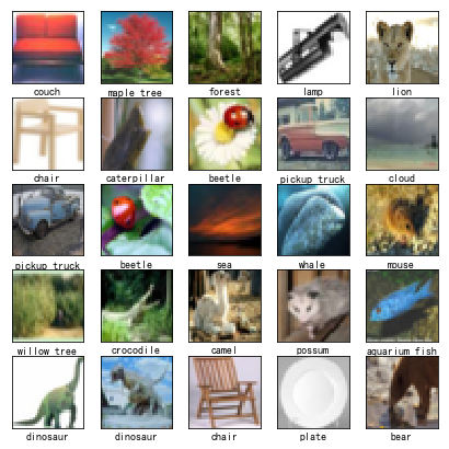

上面的大部分程式碼被我放在了 Github：https://github.com/DataLoaderX/basedataset/tree/master/loader。

總結

上面的 API 設計過程中，我發現到了許多自身的不足，不斷改進 API 的過程中，我獲得了學習和創造的喜悅。上面所介紹的 X.h5c 資料集不僅僅是那些資料集的封裝，你還可以繼續新增自己的資料集到該 資料庫中。同時，類 Loader 十分有用，它定義了一個標準，一個可以延拓到處理其他深度學習的資料集中去。

 

鄭州男科醫院

鄭州專業婦科醫院

鄭州做人流價格是多少錢

鄭州治療婦科哪家醫院好