用xgboost模型對特徵重要性進行排序

在這篇文章中，你將會學習到：

1. xgboost對預測模型特徵重要性排序的原理（即為什麼xgboost可以對預測模型特徵重要性進行排序）。
2. 如何繪製xgboost模型得到的特徵重要性條形圖。
3. 如何根據xgboost模型得到的特徵重要性，在scikit-learn進行特徵選擇。

梯度提升演算法是如何計算特徵重要性的？

使用梯度提升演算法的好處是在提升樹被建立後，可以相對直接地得到每個屬性的重要性得分。一般來說，重要性分數，衡量了特徵在模型中的提升決策樹構建中價值。一個屬性越多的被用來在模型中構建決策樹，它的重要性就相對越高。

屬性重要性是通過對資料集中的每個屬性進行計算，並進行排序得到。在單個決策書中通過每個屬性分裂點改進效能度量的量來計算屬性重要性，由節點負責加權和記錄次數。也就說一個屬性對分裂點改進效能度量越大（越靠近根節點），權值越大；被越多提升樹所選擇，屬性越重要。效能度量可以是選擇分裂節點的Gini純度，也可以是其他度量函式。

最終將一個屬性在所有提升樹中的結果進行加權求和後然後平均，得到重要性得分。

繪製特徵重要性

一個已訓練的xgboost模型能夠自動計算特徵重要性，這些重要性得分可以通過成員變數feature_importances_得到。可以通過如下命令列印：

print(model.feature_importances_)
 

我們可以直接在條形圖上繪製這些分數，以獲得資料集中每個特徵的相對重要性的直觀顯示。例如：

1. # plot

2. pyplot.bar(range(len(model.feature_importances_)), model.feature_importances_)

3. pyplot.show()

我們可以通過在the Pima Indians onset of diabetes 資料集上訓練XGBOOST模型來演示，並從計算的特徵重要性中繪製條形圖。

1. # plot feature importance manually

2. from numpy import loadtxt

3. from xgboost import XGBClassifier

4. from matplotlib import pyplot

5. # load data

6. dataset = loadtxt('pima-indians-diabetes.csv', delimiter=",")

7. # split data into X and y

8. X = dataset[:,0:8]

9. y = dataset[:,8]

10. # fit model no training data

11. model = XGBClassifier()

12. model.fit(X, y)

13. # feature importance

14. print(model.feature_importances_)

15. # plot

16. pyplot.bar(range(len(model.feature_importances_)), model.feature_importances_)

17. pyplot.show()

執行這個示例，首先的輸出特徵重要性分數：

[0.089701, 0.17109634, 0.08139535, 0.04651163, 0.10465116, 0.2026578, 0.1627907, 0.14119601]

相對重要性條形圖：

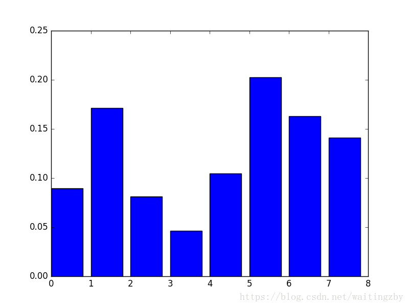
這種繪製的缺點在於，只顯示了特徵重要性而沒有排序，可以在繪製之前對特徵重要性得分進行排序。

通過內建的繪製函式進行特徵重要性得分排序後的繪製，這個函式就是plot_importance()，示例如下：

1. # plot feature importance using built-in function

2. from numpy import loadtxt

3. from xgboost import XGBClassifier

4. from xgboost import plot_importance

5. from matplotlib import pyplot

6. # load data

7. dataset = loadtxt('pima-indians-diabetes.csv', delimiter=",")

8. # split data into X and y

9. X = dataset[:,0:8]

10. y = dataset[:,8]

11. # fit model no training data

12. model = XGBClassifier()

13. model.fit(X, y)

14. # plot feature importance

15. plot_importance(model)

16. pyplot.show()

執行示例得到條形圖：

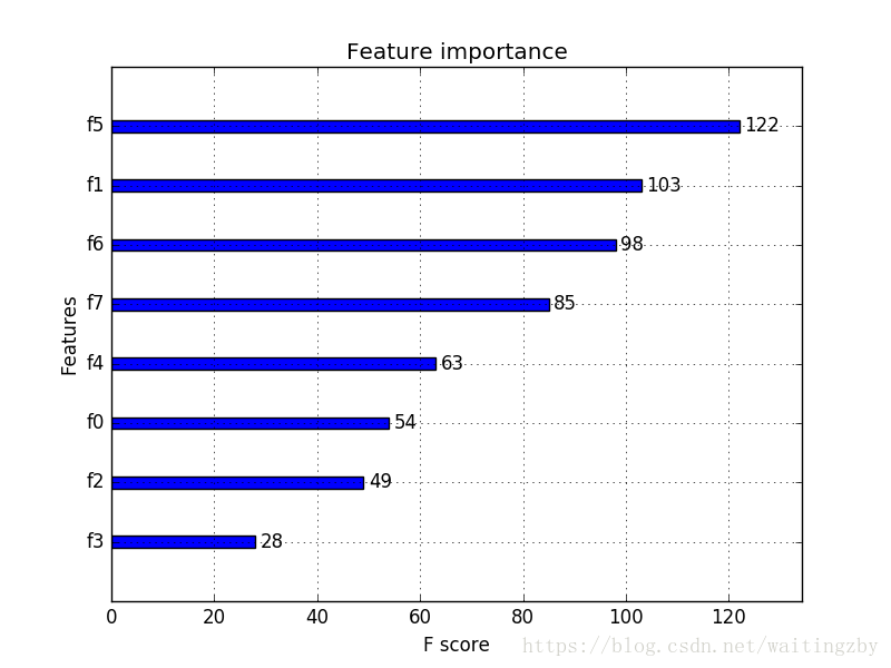
根據其在輸入陣列中的索引，特徵被自動命名為f0-f7。在問題描述中手動的將這些索引對映到名稱，我們可以看到，F5（身體質量指數）具有最高的重要性，F3（面板摺疊厚度）具有最低的重要性。

根據xgboost特徵重要性得分進行特徵選擇

特徵重要性得分，可以用於在scikit-learn中進行特徵選擇。通過SelectFromModel類實現，該類採用模型並將資料集轉換為具有選定特徵的子集。這個類可以採取預先訓練的模型，例如在整個資料集上訓練的模型。然後，它可以閾值來決定選擇哪些特徵。當在SelectFromModel例項上呼叫transform()方法時，該閾值被用於在訓練集和測試集上一致性選擇相同特徵。

在下面的示例中，我們首先在訓練集上訓練xgboost模型，然後在測試上評估。使用從訓練資料集計算的特徵重要性，然後，將模型封裝在一個SelectFromModel例項中。我們使用這個來選擇訓練集上的特徵，用所選擇的特徵子集訓練模型，然後在相同的特徵方案下對測試集進行評估。

示例：

1. # select features using threshold

2. selection = SelectFromModel(model, threshold=thresh, prefit=True)

3. select_X_train = selection.transform(X_train)

4. # train model

5. selection_model = XGBClassifier()

6. selection_model.fit(select_X_train, y_train)

7. # eval model

8. select_X_test = selection.transform(X_test)

9. y_pred = selection_model.predict(select_X_test)

我們可以通過測試多個閾值，來從特徵重要性中選擇特徵。具體而言，每個輸入變數的特徵重要性，本質上允許我們通過重要性來測試每個特徵子集。

完整示例如下：

1. # use feature importance for feature selection

2. from numpy import loadtxt

3. from numpy import sort

4. from xgboost import XGBClassifier

5. from sklearn.model_selection import train_test_split

6. from sklearn.metrics import accuracy_score

7. from sklearn.feature_selection import SelectFromModel

8. # load data

9. dataset = loadtxt('pima-indians-diabetes.csv', delimiter=",")

10. # split data into X and y

11. X = dataset[:,0:8]

12. Y = dataset[:,8]

13. # split data into train and test sets

14. X_train, X_test, y_train, y_test = train_test_split(X, Y, test_size=0.33, random_state=7)

15. # fit model on all training data

16. model = XGBClassifier()

17. model.fit(X_train, y_train)

18. # make predictions for test data and evaluate

19. y_pred = model.predict(X_test)

20. predictions = [round(value) for value in y_pred]

21. accuracy = accuracy_score(y_test, predictions)

22. print("Accuracy: %.2f%%" % (accuracy * 100.0))

23. # Fit model using each importance as a threshold

24. thresholds = sort(model.feature_importances_)

25. for thresh in thresholds:

26. # select features using threshold

27. selection = SelectFromModel(model, threshold=thresh, prefit=True)

28. select_X_train = selection.transform(X_train)

29. # train model

30. selection_model = XGBClassifier()

31. selection_model.fit(select_X_train, y_train)

32. # eval model

33. select_X_test = selection.transform(X_test)

34. y_pred = selection_model.predict(select_X_test)

35. predictions = [round(value) for value in y_pred]

36. accuracy = accuracy_score(y_test, predictions)

37. print("Thresh=%.3f, n=%d, Accuracy: %.2f%%" % (thresh, select_X_train.shape[1], accuracy*100.0))

執行示例，得到輸出：

1. Accuracy: 77.95%

2. Thresh=0.071, n=8, Accuracy: 77.95%

3. Thresh=0.073, n=7, Accuracy: 76.38%

4. Thresh=0.084, n=6, Accuracy: 77.56%

5. Thresh=0.090, n=5, Accuracy: 76.38%

6. Thresh=0.128, n=4, Accuracy: 76.38%

7. Thresh=0.160, n=3, Accuracy: 74.80%

8. Thresh=0.186, n=2, Accuracy: 71.65%

9. Thresh=0.208, n=1, Accuracy: 63.78%

我們可以看到，模型的效能通常隨著所選擇的特徵的數量而減少。在這一問題上，可以對測試集準確率和模型複雜度做一個權衡，例如選擇4個特徵，接受準確率從77.95%降到76.38%。這可能是對這樣一個小資料集的清洗，但對於更大的資料集和使用交叉驗證作為模型評估方案可能是更有用的策略。

--------------------- 本文來自 waitingzby 的CSDN 部落格 ，全文地址請點選：https://blog.csdn.net/waitingzby/article/details/81610495?utm_source=copy