
python數字圖像處理(三)邊緣檢測常用算子
在該文將介紹基本的幾種應用於邊緣檢測的濾波器,首先我們讀入saber用來做為示例的圖像
#讀入圖像代碼,在此之前應當引入必要的opencv matplotlib numpy
saber = cv2.imread("saber.png")
saber = cv2.cvtColor(saber,cv2.COLOR_BGR2RGB)
plt.imshow(saber)
plt.axis("off")
plt.show()
使用上圖作為濾波器使用的圖形
Roberts 交叉梯度算子
Roberts交叉梯度算子由兩個\(2\times2\)的模版構成,如圖。
\[
\begin{bmatrix}
-1 & 0 \ 0 & 1
\end{bmatrix}
\]
\[ \begin{bmatrix} 0 & -1 \ 1 & 0 \end{bmatrix} \]
對如圖的矩陣分別才用兩個模版相乘,並加在一起
\[
\begin{bmatrix}
Z_1 & Z_2 & Z_3 \ Z_4 & Z_5 & Z_6 \ Z_7 & Z_8 & Z_9 \\end{bmatrix}
\]
簡單表示即
\(|z_9-z_5|+|z_8-z_6|\)。
可以簡單用編程實現
首先將原圖像進行邊界擴展,並將其轉換為灰度圖。
gray_saber = cv2.cvtColor(saber,cv2.COLOR_RGB2GRAY)
gray_saber = 在接下來的的代碼中我們對圖像都會進行邊界擴展,是因為將圖像增加寬度為1的圖像能夠使在計算3*3的算子時不用考慮邊界情況
def RobertsOperator(roi):
operator_first = np.array([[-1,0],[0,1]])
operator_second = np.array([[0,-1],[1,0]])
return np.abs(np.sum(roi[1:,1:]*operator_first))+np.abs(np.sum(roi[1:,1:]*operator_second))
def Robert_saber = RobertsAlogrithm(gray_saber)plt.imshow(Robert_saber,cmap="binary")
plt.axis("off")
plt.show()
python的在這種純計算方面實在有些慢,當然這也是因為我過多的使用了for循環而沒有利用好numpy的原因
我們可以看出Roberts算子在檢測邊緣效果已經相當不錯了,但是它對噪聲相當敏感,我們給它加上噪聲在看看它的效果
噪聲代碼來源於stacksoverflow
def noisy(noise_typ,image):
    if noise_typ == "gauss":
        row,col,ch= image.shape
        mean = 0
        var = 0.1
        sigma = var**0.5
        gauss = np.random.normal(mean,sigma,(row,col,ch))
        gauss = gauss.reshape(row,col,ch)
        noisy = image + gauss
        return noisy
    elif noise_typ == "s&p":
        row,col,ch = image.shape
        s_vs_p = 0.5
        amount = 0.004
        out = np.copy(image)
        num_salt = np.ceil(amount * image.size * s_vs_p)
        coords = [np.random.randint(0, i - 1, int(num_salt))
              for i in image.shape]
        out[coords] = 1
        num_pepper = np.ceil(amount* image.size * (1. - s_vs_p))
        coords = [np.random.randint(0, i - 1, int(num_pepper)) for i in image.shape]
        out[coords] = 0
        return out
    elif noise_typ == "poisson":
        vals = len(np.unique(image))
        vals = 2 ** np.ceil(np.log2(vals))
        noisy = np.random.poisson(image * vals) / float(vals)
        return noisy
    elif noise_typ =="speckle":
        row,col,ch = image.shape
        gauss = np.random.randn(row,col,ch)
        gauss = gauss.reshape(row,col,ch)
        noisy = image + image * gauss
        return noisy
dst = noisy("s&p",saber)
plt.subplot(121)
plt.title("add noise")
plt.axis("off")
plt.imshow(dst)
plt.subplot(122)
dst = cv2.cvtColor(dst,cv2.COLOR_RGB2GRAY)
plt.title("Robert Process")
plt.axis("off")
dst = RobertsAlogrithm(dst)
plt.imshow(dst,cmap="binary")
plt.show()
這裏我們可以看出Robert算子對於噪聲過於敏感,在加了噪聲後,人的邊緣變得非常不清晰
Prewitt算子
Prewitt算子是一種\(3\times3\)模板的算子,它有兩種形式,分別表示水平和垂直的梯度.
垂直梯度
\[
\begin{bmatrix}
-1 & -1 & -1 \ 0 & 0 & 0 \ 1 & 1 & 1 \\end{bmatrix}
\]
水平梯度
\[
\begin{bmatrix}
-1 & 0 & 1 \ -1 & 0 & 1 \ -1 & 0 & 1 \\end{bmatrix}
\]
對於如圖的矩陣起始值
\[
\begin{bmatrix}
Z_1 & Z_2 & Z_3 \ Z_4 & Z_5 & Z_6 \ Z_7 & Z_8 & Z_9 \\end{bmatrix}
\]
就是以下兩個式子
\[
|(z_7+z_8+z_9)-(z_1+z_2+z_3)|
\]
\[
|(z_1+z_4+z_7)-(z_3+z_6+z_9)|
\]
1與-1更換位置對結果並不會產生影響
def PreWittOperator(roi,operator_type):
    if operator_type == "horizontal":
        prewitt_operator = np.array([[-1,-1,-1],[0,0,0],[1,1,1]])
    elif operator_type == "vertical":
        prewitt_operator = np.array([[-1,0,1],[-1,0,1],[-1,0,1]])
    else:
        raise("type Error")
    result = np.abs(np.sum(roi*prewitt_operator))
    return result

def PreWittAlogrithm(image,operator_type):
    new_image = np.zeros(image.shape)
    image = cv2.copyMakeBorder(image,1,1,1,1,cv2.BORDER_DEFAULT)
    for i in range(1,image.shape[0]-1):
        for j in range(1,image.shape[1]-1):
            new_image[i-1,j-1] = PreWittOperator(image[i-1:i+2,j-1:j+2],operator_type)
    new_image = new_image*(255/np.max(image))
    return new_image.astype(np.uint8)
在PreWitt算子執行中要考慮大於255的情況,使用下面代碼
new_image = new_image*(255/np.max(image))將其放縮到0-255之間,並使用astype將其轉換到uint8類型
plt.subplot(121)
plt.title("horizontal")
plt.imshow(PreWittAlogrithm(gray_saber,"horizontal"),cmap="binary")
plt.axis("off")
plt.subplot(122)
plt.title("vertical")
plt.imshow(PreWittAlogrithm(gray_saber,"vertical"),cmap="binary")
plt.axis("off")
plt.show()
現在我們看一下Prewitt對噪聲的敏感性
dst = noisy("s&p",saber)
plt.subplot(131)
plt.title("add noise")
plt.axis("off")
plt.imshow(dst)

plt.subplot(132)
plt.title("Prewitt Process horizontal")
plt.axis("off")
plt.imshow(PreWittAlogrithm(gray_saber,"horizontal"),cmap="binary")

plt.subplot(133)
plt.title("Prewitt Process vertical")
plt.axis("off")
plt.imshow(PreWittAlogrithm(gray_saber,"vertical"),cmap="binary")
plt.show()
選擇水平梯度或垂直梯度從上圖可以看出對於邊緣的影響還是相當大的.
Sobel算子
Sobel算子根據像素點上下、左右鄰點灰度加權差,在邊緣處達到極值這一現象檢測邊緣。對噪聲具有平滑作用,提供較為精確的邊緣方向信息,邊緣定位精度不夠高。當對精度要求不是很高時,是一種較為常用的邊緣檢測方法。相比Prewitt他周邊像素對於判斷邊緣的貢獻是不同的.
垂直梯度
\[
\begin{bmatrix}
-1 & -2 & -1 \ 0 & 0 & 0 \ 1 & 2 & 1 \\end{bmatrix}
\]
水平梯度
\[
\begin{bmatrix}
-1 & 0 & 1 \ -2 & 0 & 2 \ -1 & 0 & 1 \\end{bmatrix}
\]
對上面的代碼稍微修改算子即可
def SobelOperator(roi,operator_type):
    if operator_type == "horizontal":
        sobel_operator = np.array([[-1,-2,-1],[0,0,0],[1,2,1]])
    elif operator_type == "vertical":
        sobel_operator = np.array([[-1,0,1],[-2,0,2],[-1,0,1]])
    else:
        raise("type Error")
    result = np.abs(np.sum(roi*sobel_operator))
    return result

def SobelAlogrithm(image,operator_type):
    new_image = np.zeros(image.shape)
    image = cv2.copyMakeBorder(image,1,1,1,1,cv2.BORDER_DEFAULT)
    for i in range(1,image.shape[0]-1):
        for j in range(1,image.shape[1]-1):
            new_image[i-1,j-1] = SobelOperator(image[i-1:i+2,j-1:j+2],operator_type)
    new_image = new_image*(255/np.max(image))
return new_image.astype(np.uint8)plt.subplot(121)
plt.title("horizontal")
plt.imshow(SobelAlogrithm(gray_saber,"horizontal"),cmap="binary")
plt.axis("off")
plt.subplot(122)
plt.title("vertical")
plt.imshow(SobelAlogrithm(gray_saber,"vertical"),cmap="binary")
plt.axis("off")
plt.show()
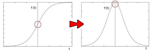
無論是Sobel還是Prewitt其實是求了單個方向顏色變化的極值
在某個方向上顏色的變化如圖(此圖來源於opencv官方文檔)
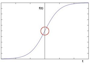
對其求導可以得到這樣一條曲線
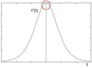
由此我們可以得知邊緣可以通過定位梯度值大於鄰域的相素的方法找到(或者推廣到大於一個閥值).
而Sobel就是利用了這一定理
Laplace算子
無論是Sobel還是Prewitt都是求單方向上顏色變化的一階導(Sobel相比Prewitt增加了權重),那麽如何才能反映空間上的顏色變化的一個極值呢?
我們試著在對邊緣求一次導
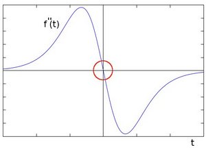
在一階導數的極值位置,二階導數為0。所以我們也可以用這個特點來作為檢測圖像邊緣的方法。 但是, 二階導數的0值不僅僅出現在邊緣(它們也可能出現在無意義的位置),但是我們可以過濾掉這些點。
在實際情況中我們不可能用0作為判斷條件,而是設定一個閾值,這就引出來Laplace算子
\begin{bmatrix}
0 & 1 & 0 \
1 & -4 & 1 \
0 & 1 & 0 \
\end{bmatrix}
\begin{bmatrix}
1 & 1 & 1 \
1 & -8 & 1 \
1 & 1 & 1 \
\end{bmatrix}
def LaplaceOperator(roi,operator_type):
    if operator_type == "fourfields":
        laplace_operator = np.array([[0,1,0],[1,-4,1],[0,1,0]])
    elif operator_type == "eightfields":
        laplace_operator = np.array([[1,1,1],[1,-8,1],[1,1,1]])
    else:
        raise("type Error")
    result = np.abs(np.sum(roi*laplace_operator))
    return result

def LaplaceAlogrithm(image,operator_type):
    new_image = np.zeros(image.shape)
    image = cv2.copyMakeBorder(image,1,1,1,1,cv2.BORDER_DEFAULT)
    for i in range(1,image.shape[0]-1):
        for j in range(1,image.shape[1]-1):
            new_image[i-1,j-1] = LaplaceOperator(image[i-1:i+2,j-1:j+2],operator_type)
    new_image = new_image*(255/np.max(image))
return new_image.astype(np.uint8)plt.subplot(121)
plt.title("fourfields")
plt.imshow(LaplaceAlogrithm(gray_saber,"fourfields"),cmap="binary")
plt.axis("off")
plt.subplot(122)
plt.title("eightfields")
plt.imshow(LaplaceAlogrithm(gray_saber,"eightfields"),cmap="binary")
plt.axis("off")
plt.show()
上圖為比較取值不同的laplace算子實現的區別.
Canny算子
Canny邊緣檢測算子是一種多級檢測算法。1986年由John F. Canny提出,同時提出了邊緣檢測的三大準則:
- 低錯誤率的邊緣檢測:檢測算法應該精確地找到圖像中的盡可能多的邊緣,盡可能的減少漏檢和誤檢。
- 最優定位:檢測的邊緣點應該精確地定位於邊緣的中心。
- 圖像中的任意邊緣應該只被標記一次,同時圖像噪聲不應產生偽邊緣。
Canny邊緣檢測算法的實現較為復雜,主要分為以下步驟,
- 高斯模糊
- 計算梯度幅值和方向
- 非極大值 抑制
- 滯後閾值
高斯模糊
在前面的章節中已經實現過均值模糊,模糊在圖像處理中經常用來去除一些無關的細節.
均值模糊引出了另一個思考,周邊每個像素點的權重設為一樣是否合適?
(周邊像素點的權重是很多算法的區別,比如Sobel和Prewitt)
因此概率中非常熟悉的正態分布函數便被引入.正太分布函數的密度函數就是高斯函數,使用高斯函數來給周邊像素點分配權重.
更詳細的可以參考高斯模糊的算法
在opencv的官方文檔中它介紹了這樣一個\(5\times5\)的高斯算子
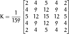
相比直接的使用密度函數來分配權重,Opencv介紹的高斯算子是各像素點乘以一個大於1的比重,最後乘以一個\(1 \frac {159}\),其實就是歸一化的密度函數.這有效避免了計算機計算的精度問題

我們在此處直接使用\(3\times3\)的算子

我們將其歸一化然後代入上面的代碼即可
def GaussianOperator(roi):
    GaussianKernel = np.array([[1,2,1],[2,4,2],[1,2,1]])
    result = np.sum(roi*GaussianKernel/16)
    return result

def GaussianSmooth(image):
    new_image = np.zeros(image.shape)
    image = cv2.copyMakeBorder(image,1,1,1,1,cv2.BORDER_DEFAULT)
    for i in range(1,image.shape[0]-1):
        for j in range(1,image.shape[1]-1):
            new_image[i-1,j-1] =GaussianOperator(image[i-1:i+2,j-1:j+2])
    return new_image.astype(np.uint8)
smooth_saber = GaussianSmooth(gray_saber)
plt.subplot(121)
plt.title("Origin Image")
plt.axis("off")
plt.imshow(gray_saber,cmap="gray")
plt.subplot(122)
plt.title("GaussianSmooth Image")
plt.axis("off")
plt.imshow(smooth_saber,cmap="gray")
plt.show()
計算梯度幅值和方向
我們知道邊緣實質是顏色變換的極值,可能出現在各個方向上,因此能否在計算時考慮多個方向的梯度,是算法效果優異的體現之一
在之前的Sobel等算子中我們將水平和垂直方向是分開考慮的.在Canny算子中利用下面公式將多個方向都考慮到
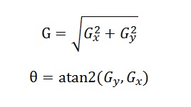
Gx = SobelAlogrithm(smooth_saber,"horizontal")
Gy = SobelAlogrithm(smooth_saber,"vertical")
G = np.sqrt(np.square(Gx.astype(np.float64))+np.square(Gy.astype(np.float64)))
cita = np.arctan2(Gy.astype(np.float64),Gx.astype(np.float64))cita求出了圖像每一個點的梯度,在之後的非極大值抑制中會有作用
plt.imshow(G.astype(np.uint8),cmap="gray")
plt.axis("off")
plt.show()
我們發現對於圖像使用sobel算子使得獲得的邊緣較粗,下一步我們將使圖像的線條變細
非最大值抑制
在獲得梯度的方向和大小之後,應該對整幅圖想做一個掃描,出去那些非邊界上的點。對每一個像素進行檢查,看這個點的梯度是不是周圍具有相同梯度方向的點中最大的。
(圖像來源於opencv官方文檔)

非極大值的算法實現非常簡單
- 比較當前點的梯度強度和正負梯度方向點的梯度強度。
- 如果當前點的梯度強度和同方向的其他點的梯度強度相比較是最大,保留其值。否則抑制,即設為0。比如當前點的方向指向正上方90°方向,那它需要和垂直方向,它的正上方和正下方的像素比較。
def NonmaximumSuppression(image,cita):
    keep = np.zeros(cita.shape)
    cita = np.abs(cv2.copyMakeBorder(cita,1,1,1,1,cv2.BORDER_DEFAULT))
    for i in range(1,cita.shape[0]-1):
        for j in range(1,cita.shape[1]-1):
            if cita[i][j]>cita[i-1][j] and cita[i][j]>cita[i+1][j]:
                keep[i-1][j-1] = 1
            elif cita[i][j]>cita[i][j+1] and cita[i][j]>cita[i][j-1]:
                keep[i-1][j-1] = 1
            elif cita[i][j]>cita[i+1][j+1] and cita[i][j]>cita[i-1][j-1]:
                keep[i-1][j-1] = 1
            elif cita[i][j]>cita[i-1][j+1] and cita[i][j]>cita[i+1][j-1]:
                keep[i-1][j-1] = 1
            else:
                keep[i-1][j-1] = 0
    return keep*image
這裏的代碼我們先創建了一個keep矩陣,凡是在cita中梯度大於周邊的點設為1,否則設為0,然後與原圖相乘.(這是我想得比較巧妙的一個方法)
nms_image = NonmaximumSuppression(G,cita)
nms_image = (nms_image*(255/np.max(nms_image))).astype(np.uint8)plt.imshow(nms_image,cmap="gray")
plt.axis("off")
plt.show()
在上面的極大值抑制中我們使邊緣的線變得非常細,但是仍然有相當多的小點,得使用一種算法將他們去除
滯後閾值
滯後閾值的算法如下
Canny 使用了滯後閾值,滯後閾值需要兩個閾值(高閾值和低閾值):
- 如果某一像素位置的幅值超過 高 閾值, 該像素被保留為邊緣像素。
- 如果某一像素位置的幅值小於 低 閾值, 該像素被排除。
- 如果某一像素位置的幅值在兩個閾值之間,該像素僅僅在連接到一個高於 高 閾值的像素時被保留。
在opencv官方文檔中推薦我們用2:1或3:1的高低閾值.
我們使用3:1的閾值來進行滯後閾值算法.
滯後閾值的算法可以分成兩步首先使用最大閾值,最小閾值排除掉部分點.
MAXThreshold = np.max(nms_image)/4*3
MINThreshold = np.max(nms_image)/4
usemap = np.zeros(nms_image.shape)
high_list = []
for i in range(nms_image.shape[0]):
for j in range(nms_image.shape[1]):
if nms_image[i,j]>MAXThreshold:
high_list.append((i,j))direct = [(0,1),(1,1),(-1,1),(-1,-1),(1,-1),(1,0),(-1,0),(0,-1)]
def DFS(stepmap,start):
route = [start]
while route:
now = route.pop()
if usemap[now] == 1:
break
usemap[now] = 1
for dic in direct:
next_coodinate = (now[0]+dic[0],now[1]+dic[1])
if not usemap[next_coodinate] and nms_image[next_coodinate]>MINThreshold \
and next_coodinate[0]<stepmap.shape[0]-1 and next_coodinate[0]>=0 \
and next_coodinate[1]<stepmap.shape[1]-1 and next_coodinate[1]>=0:
route.append(next_coodinate)for i in high_list:
DFS(nms_image,i)plt.imshow(nms_image*usemap,cmap="gray")
plt.axis("off")
plt.show()
可以發現這次的效果並不好,這是由於最大最小閾值設定不是很好導致的,我們將上面代碼整理,將最大閾值,最小閾值改為可變參數,調參來優化效果.
Canny邊緣檢測代碼
def CannyAlogrithm(image,MINThreshold,MAXThreshold):
image = GaussianSmooth(image)
Gx = SobelAlogrithm(image,"horizontal")
Gy = SobelAlogrithm(image,"vertical")
G = np.sqrt(np.square(Gx.astype(np.float64))+np.square(Gy.astype(np.float64)))
G = G*(255/np.max(G)).astype(np.uint8)
cita = np.arctan2(Gy.astype(np.float64),Gx.astype(np.float64))
nms_image = NonmaximumSuppression(G,cita)
nms_image = (nms_image*(255/np.max(nms_image))).astype(np.uint8)
usemap = np.zeros(nms_image.shape)
high_list = []
for i in range(nms_image.shape[0]):
    for j in range(nms_image.shape[1]):
        if nms_image[i,j]>MAXThreshold:
            high_list.append((i,j))
direct = [(0,1),(1,1),(-1,1),(-1,-1),(1,-1),(1,0),(-1,0),(0,-1)]
def DFS(stepmap,start):
route = [start]
while route:
now = route.pop()
if usemap[now] == 1:
break
usemap[now] = 1
for dic in direct:
next_coodinate = (now[0]+dic[0],now[1]+dic[1])
if next_coodinate[0]<stepmap.shape[0]-1 and next_coodinate[0]>=0 \
and next_coodinate[1]<stepmap.shape[1]-1 and next_coodinate[1]>=0 \
and not usemap[next_coodinate] and nms_image[next_coodinate]>MINThreshold:
route.append(next_coodinate)
for i in high_list:
    DFS(nms_image,i)
return nms_image*usemap我們試著調整閾值,來對其他圖片進行檢測


通過調整閾值可以減少毛點的存在,控制線的清晰
(PS:在使用canny過程中為了減少python運算的時間,我將圖片進行了縮放,這也導致了效果不夠明顯,canny邊緣檢測在高分辨率情況下效果會更好)
參考資料
Opencv文檔
stackoverflow
Numpy設計的是如此出色,以至於在實現算法時我能夠忽略如此之多無關的細節
python數字圖像處理(三)邊緣檢測常用算子