• 聚類（clustering）

　　用於找出不帶標簽數據的相似性的算法

• K-Means聚類算法簡介

　　與廣義線性模型和決策樹類似，K-Means參 數的最優解也是以成本函數最小化為目標。K-Means成本函數公式如下：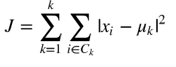

　　成本函數是各個類畸變程度（distortions）之和。每個類的畸變程度等於 該類重心與其內部成員位置距離的平方和。若類內部的成員彼此間越緊湊則類的畸變程度越小，反 之，若類內部的成員彼此間越分散則類的畸變程度越大。求解成本函數最小化的參數就是一個重復配 置每個類包含的觀測值，並不斷移動類重心的過程。首先，類的重心是隨機確定的位置。實際上，重 心位置等於隨機選擇的觀測值的位置。每次叠代的時候，K-Means會把觀測值分配到離它們最近的 類，然後把重心移動到該類全部成員位置的平均值那裏。

import matplotlib.pyplot as plt
from matplotlib.font_manager import FontProperties
font = FontProperties(fname=r"C:\Users\Lenovo\Desktop\data_set\msyh.ttc", size=10)

‘‘‘可視化樣本點‘‘‘
import numpy as np
X0 = np.array([7, 5, 7, 3, 4, 1, 0, 2, 8, 6, 5, 3])
X1 = np.array([5, 7, 7, 3, 6, 4, 0, 2, 7, 8, 5, 7])
plt.figure()
plt.axis([
 
-1, 9, -1, 9])
plt.grid(True)
plt.plot(X0, X1, ‘k.‘)
# plt.show()

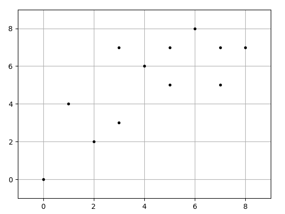
C1 = [1, 4, 5, 9, 11]
C2 = list(set(range(12)) - set(C1))
X0C1, X1C1 = X0[C1], X1[C1]
X0C2, X1C2 = X0[C2], X1[C2]
plt.figure()
plt.title(‘第一次叠代後聚類結果‘,fontproperties=font)
plt.axis([-1, 9, -1, 9])
plt.grid(True)
plt.plot(X0C1, X1C1, ‘rx‘
 
)
plt.plot(X0C2, X1C2, ‘g.‘)
plt.plot(4,6,‘rx‘,ms=12.0)
plt.plot(5,5,‘g.‘,ms=12.0)
plt.show()

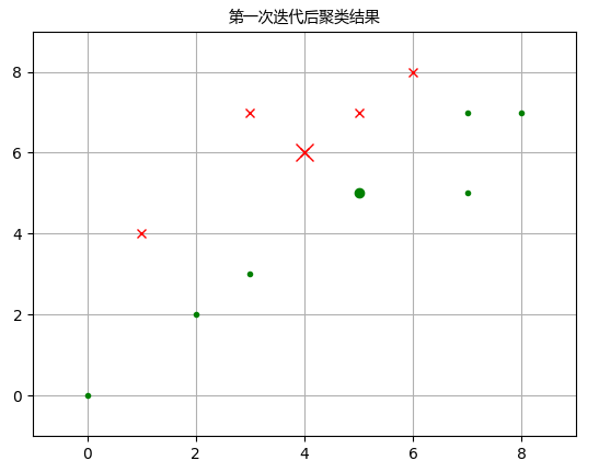
C1 = [1, 2, 4, 8, 9, 11]
C2 = list(set(range(12)) - set(C1))
X0C1, X1C1 = X0[C1], X1[C1]
X0C2, X1C2 = X0[C2], X1[C2]
plt.figure()
plt.title(‘第二次叠代後聚類結果‘,fontproperties=font)
plt.axis([-1, 9, -1, 9])
plt.grid(True)
plt.plot(X0C1, X1C1, ‘rx‘)
plt.plot(X0C2, X1C2, ‘g.‘)
plt.plot(3.8,6.4,‘rx‘,ms=12.0)
plt.plot(4.57,4.14,‘g.‘,ms=12.0)
plt.show()

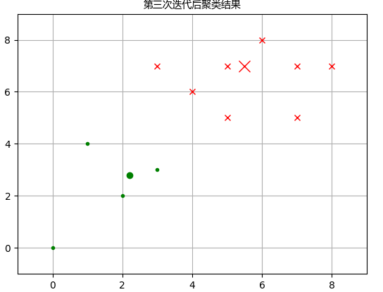
C1 = [0, 1, 2, 4, 8, 9, 10, 11]
C2 = list(set(range(12)) - set(C1))
X0C1, X1C1 = X0[C1], X1[C1]
X0C2, X1C2 = X0[C2], X1[C2]
plt.figure()
plt.title(‘第三次叠代後聚類結果‘,fontproperties=font)
plt.axis([-1, 9, -1, 9])
plt.grid(True)
plt.plot(X0C1, X1C1, ‘rx‘)
plt.plot(X0C2, X1C2, ‘g.‘)
plt.plot(5.5,7.0,‘rx‘,ms=12.0)
plt.plot(2.2,2.8,‘g.‘,ms=12.0)
plt.show()

• 局部最優解

• 肘部法則

import numpy as np
cluster1 = np.random.uniform(0.5, 1.5, (2, 10))
cluster2 = np.random.uniform(3.5, 4.5, (2, 10))
X = np.hstack((cluster1, cluster2)).T
# plt.figure()
# plt.axis([0, 5, 0, 5])
# plt.grid(True)
# plt.plot(X[:,0],X[:,1],‘k.‘)

‘‘‘計算K值從1到10對應的平均畸變程度：‘‘‘
from sklearn.cluster import KMeans
from scipy.spatial.distance import cdist
K = range(1, 11)
# K = list(range(1, 11))
meandistortions = []
for k in K:
    kmeans = KMeans(n_clusters=k)
    kmeans.fit(X)
    meandistortions.append(sum(np.min(cdist(X,kmeans.cluster_centers_,‘euclidean‘), axis=1))
                           / X.shape[0])
plt.plot(K, meandistortions, ‘bx-‘)
plt.xlabel(‘k‘)
plt.ylabel(‘平均畸變程度‘,fontproperties=font)
plt.title(‘用肘部法則來確定最佳的K值‘,fontproperties=font)
plt.show()

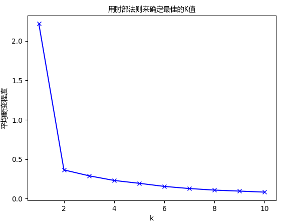
從圖中可以看出，K值從1到2時，平均畸變程度變化最大。超過2以後，平均畸變程度變化顯著降 低。因此肘部就是K=2.

下面用肘部法則來確定3個類的最佳的K值：

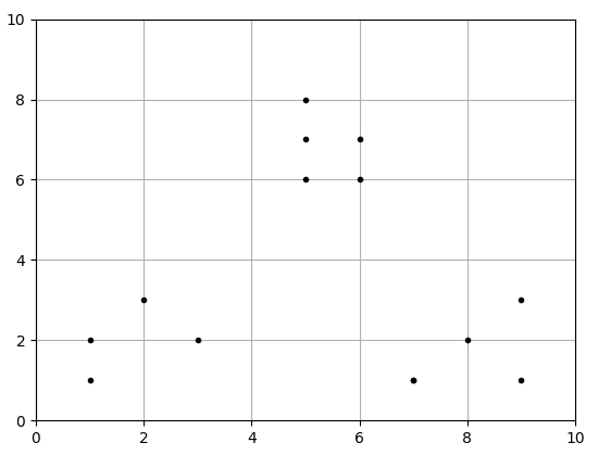
import numpy as np
x1 = np.array([1, 2, 3, 1, 5, 6, 5, 5, 6, 7, 8, 9, 7, 9])
x2 = np.array([1, 3, 2, 2, 8, 6, 7, 6, 7, 1, 2, 1, 1, 3])
X = np.array(list(zip(x1, x2))).reshape(len(x1), 2)
# print(list(zip(x1, x2)))
# print(X)
plt.figure()
plt.axis([0, 10, 0, 10])
plt.grid(True)
plt.plot(X[:,0],X[:,1],‘k.‘)
plt.show()

from sklearn.cluster import KMeans
from scipy.spatial.distance import cdist
K = range(1, 10)
meandistortions = []
for k in K:
    kmeans = KMeans(n_clusters=k)
    kmeans.fit(X)
    meandistortions.append(sum(np.min(cdist(X, kmeans.cluster_centers_, ‘euclidean‘),
                                      axis=1)) / X.shape[0])
plt.plot(K, meandistortions, ‘bx-‘)
plt.xlabel(‘k‘)
plt.ylabel(‘平均畸變程度‘,fontproperties=font)
plt.title(‘用肘部法則來確定最佳的K值‘,fontproperties=font)
plt.show()

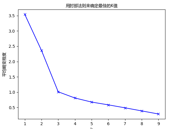
從圖中可以看出， 值從1到3時，平均畸變程度變化最大。超過3以後，平均畸變程度變化顯著降低。因此肘部就是 。

• 聚類效果評估
• 聚類算法效果評估方法稱為輪廓系數（Silhouette Coefficient)

計算公式如下：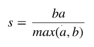

a是每一個類中樣本彼此距離的均值，b 是一個類中樣本與其最近的那個類的所有樣本的距離的均 值。下面的例子運行四次K-Means，從一個數據集中分別創建2，3，4，5，8個類，然後分別計算它們 的輪廓系數。

import matplotlib.pyplot as plt
from matplotlib.font_manager import FontProperties
font = FontProperties(fname=r"C:\Users\Lenovo\Desktop\data_set\msyh.ttc", size=10)

import numpy as np
from sklearn.cluster import KMeans
from sklearn import metrics
plt.figure(figsize=(6, 6))
plt.subplot(3, 2, 1)
x1 = np.array([1, 2, 3, 1, 5, 6, 5, 5, 6, 7, 8, 9, 7, 9])
x2 = np.array([1, 3, 2, 2, 8, 6, 7, 6, 7, 1, 2, 1, 1, 3])
X = np.array(list(zip(x1, x2))).reshape(len(x1), 2)
plt.xlim([0, 10])
plt.ylim([0, 10])
plt.title(‘樣本‘,fontproperties=font)
plt.scatter(x1, x2)
colors = [‘b‘, ‘g‘, ‘r‘, ‘c‘, ‘m‘, ‘y‘, ‘k‘, ‘b‘]
markers = [‘o‘, ‘s‘, ‘D‘, ‘v‘, ‘^‘, ‘p‘, ‘*‘, ‘+‘]
tests = [2, 3, 4, 5, 8]
subplot_counter = 1
for t in tests:
    subplot_counter += 1
    plt.subplot(3, 2, subplot_counter)
    kmeans_model = KMeans(n_clusters=t).fit(X)
    ‘‘‘kmeans_model.labels_獲取索引及對應的類別‘‘‘
    for i, l in enumerate(kmeans_model.labels_):
        plt.tight_layout()  #用來調整子圖間距
        plt.plot(x1[i], x2[i], color=colors[l], marker=markers[l],ls=‘None‘)
        plt.xlim([0, 10])
        plt.ylim([0, 10])
        plt.title(‘K = %s, 輪廓系數 = %.03f‘
                  % (t, metrics.silhouette_score(X, kmeans_model.labels_,
                                                 metric=‘euclidean‘)),
                  fontproperties=font)
plt.show()

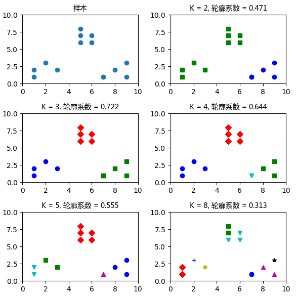
很顯然，這個數據集包括三個類。在K=3 的時候輪廓系數是最大的。在 K=8的時候，每個類的 樣本不僅彼此很接近，而且與其他類的樣本也非常接近，因此這時輪廓系數是最小的。
Re：如果是高維就要通過降維可視化分析

K-Means聚類